Introduction to Neural Networks
1. Overview
Neural networks are a type of machine learning model inspired by the structure and function of the human brain. They are widely used in various fields and have shown great success in solving complex problems.
In this lab, we will explore the basics of neural networks, their applications, and the typical workflow involved in building and training neural networks.
2. Neural Networks
A neural network is composed of interconnected nodes, called neurons, organized in layers. Each neuron takes inputs, performs computations, and produces an output. The connections between neurons are represented by weights, which determine the strength of the influence of one neuron on another.
Neural networks can be used for various tasks, including classification, regression, and pattern recognition. They have been successfully applied in image and speech recognition, natural language processing, recommendation systems, and many other domains.
 Source: 3Blue1Brown.
3. Workflow
The typical workflow for working with neural networks involves the following steps:
Data Preparation: Collect and preprocess the data for training and testing the neural network.
Model Architecture: Design the structure of the neural network, including the number of layers, types of activation functions, and the number of neurons in each layer.
Model Compilation: Configure the model by specifying the loss function, optimizer, and evaluation metrics.
Model Training: Train the neural network on the training data, adjusting the weights and biases to minimize the loss function.
Model Evaluation: Evaluate the performance of the trained model on the test data using appropriate metrics.
Model Deployment: Deploy the trained model to make predictions on new, unseen data.
Throughout this lab, we will take a look at each step of the workflow to see what we will be capable of by the end of these labs. Let's get started!
3.1. Data Preparation
Data preparation is an essential step in building and training neural networks. It involves collecting and preprocessing the data to ensure that it is in a suitable format for training and testing the neural network.3.1.1. Data Collection
The first step in data preparation is to collect the necessary data for training and testing the neural network. This may involve gathering data from various sources, such as databases, APIs, or files.
3.1.2. Data Cleaning
Once the data is collected, it is important to clean the data to remove any inconsistencies, errors, or missing values. This may involve techniques such as removing duplicates, handling missing data, and correcting any errors in the data.
3.1.3. Data Transformation
After cleaning the data, it may be necessary to transform the data into a format that is suitable for training the neural network. This may involve techniques such as scaling the data, encoding categorical variables, or normalizing the data.
3.1.4. Data Splitting
To evaluate the performance of the neural network, it is common to split the data into training and testing sets. The training set is used to train the neural network, while the testing set is used to evaluate its performance. This helps to assess how well the neural network generalizes to unseen data.
3.1.5. Data Augmentation
In some cases, it may be beneficial to augment the data by generating additional training examples. This can help to increase the diversity of the training data and improve the performance of the neural network.
3.1.6. Example
import torch
import torchvision
from torchvision import transforms

# Define the transformations to apply to the dataset
transform = transforms.Compose([
	transforms.RandomRotation(10),  # Apply random rotation
	transforms.RandomAffine(0, translate=(0.1, 0.1)),  # Apply random affine transformation
	transforms.ToTensor(),  # Convert the image to a tensor
	transforms.Normalize((0.5,), (0.5,))  # Normalize the image
])

# Load the MNIST dataset
train_dataset = torchvision.datasets.MNIST(root='./data', train=True, download=True, transform=transform)

# Split the training dataset into training and validation sets
train_size = int(0.8 * len(train_dataset))
val_size = len(train_dataset) - train_size
train_dataset, val_dataset = torch.utils.data.random_split(train_dataset, [train_size, val_size])

# Load the test dataset
test_dataset = torchvision.datasets.MNIST(root='./data', train=False, download=True, transform=transform)

# Create data loaders for training, validation, and testing
train_loader = torch.utils.data.DataLoader(train_dataset, batch_size=64, shuffle=True)
val_loader = torch.utils.data.DataLoader(val_dataset, batch_size=64, shuffle=False)
test_loader = torch.utils.data.DataLoader(test_dataset, batch_size=64, shuffle=False)
Overall, data preparation is a crucial step in building and training neural networks. It ensures that the data is in a suitable format and quality for training the neural network effectively.
3.2. Neural Network Model Architecture
Designing the structure of a neural network involves determining the number of layers, the types of activation functions, and the number of neurons in each layer. These choices greatly impact the performance and capabilities of the neural network.3.2.1. Number of Layers
The number of layers in a neural network is an important consideration. Generally, neural networks consist of an input layer, one or more hidden layers, and an output layer. The number of hidden layers can vary depending on the complexity of the problem being solved. Adding more layers can potentially improve the network's ability to learn complex patterns, but it also increases the risk of overfitting.
3.2.2. Activation Functions
Activation functions introduce non-linearity to the neural network, allowing it to learn and model complex relationships between inputs and outputs. Common activation functions include:
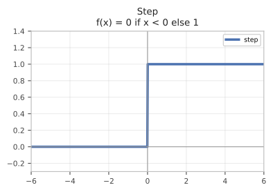
Step Function: The step function is a simple activation function that outputs a binary value based on a threshold. It returns 0 if the input is less than the threshold, and 1 otherwise. The step function is often used in binary classification problems.
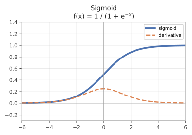
Sigmoid: Sigmoid is often used in the output layer for binary classification problems. It squashes the output between 0 and 1, representing the probability of the positive class.
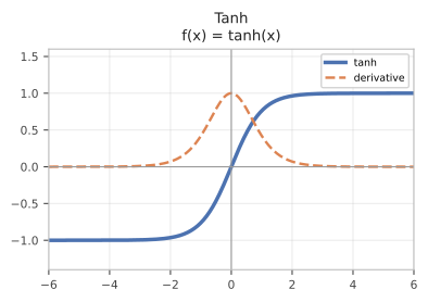
Tanh (Hyperbolic Tangent): The tanh function is a popular activation function that squashes the input values between -1 and 1. It is symmetric around the origin and is useful for capturing non-linear relationships in the data.
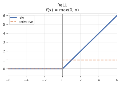
ReLU (Rectified Linear Unit): ReLU is a popular choice for hidden layers. It sets all negative values to zero and keeps positive values unchanged.
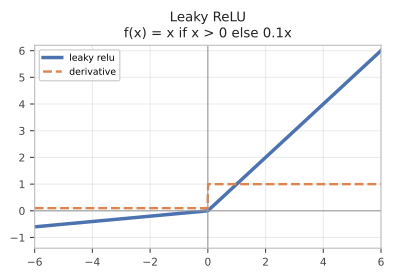
LReLU (Leaky ReLU): The Leaky ReLU is a variation of the ReLU activation function that allows small negative values instead of setting them to zero. This helps to mitigate the "dying ReLU" problem, where neurons can become inactive and stop learning.
Softmax: Softmax is commonly used in the output layer for multi-class classification problems. It normalizes the outputs into a probability distribution over the classes.
These activation functions can be used in different layers of the neural network depending on the problem and the desired behavior of the network.
| Step | Sigmoid | Tanh |
 |
 |
 |
| ReLU | LReLU | Softmax |
 |
 |
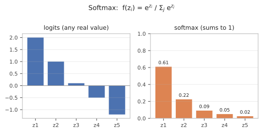 |
Diagram redrawn locally; the original was hot-linked and is no longer served.
3.2.3. Number of Neurons in Each Layer
The number of neurons in each layer determines the capacity and complexity of the neural network. The input layer should have the same number of neurons as the number of features in the input data. The number of neurons in the hidden layers can vary depending on the problem complexity and the amount of data available. The output layer should have the same number of neurons as the number of classes in the classification problem.
It is important to strike a balance between too few and too many neurons in each layer. Too few neurons may result in underfitting, where the network fails to capture the complexity of the data. Too many neurons may lead to overfitting, where the network memorizes the training data but fails to generalize to new data.
3.2.4. Example
import torch.nn as nn

# Define the neural network architecture
class SimpleNet(nn.Module):
    def __init__(self, input_size, hidden_size, output_size):
        super(SimpleNet, self).__init__()
        self.fc1 = nn.Linear(input_size, hidden_size)
        self.relu = nn.ReLU()
        self.sigmoid = nn.Sigmoid()
        self.tanh = nn.Tanh()
        self.fc2 = nn.Linear(hidden_size, output_size)

    def forward(self, x):
        # MNIST arrives as (batch, 1, 28, 28); a Linear layer wants (batch, features)
        x = x.view(x.size(0), -1)
        out = self.fc1(x)
        out = self.relu(out)
        out = self.sigmoid(out)
        out = self.tanh(out)
        out = self.fc2(out)
        return out

# Create an instance of the neural network.
# The input layer must match the number of features in the data (28 * 28 pixels),
# and the output layer must match the number of classes (10 digits).
input_size = 28 * 28
hidden_size = 128
output_size = 10
model = SimpleNet(input_size, hidden_size, output_size)

# Print the model architecture
print(model)
SimpleNet(
  (fc1): Linear(in_features=784, out_features=128, bias=True)
  (relu): ReLU()
  (sigmoid): Sigmoid()
  (tanh): Tanh()
  (fc2): Linear(in_features=128, out_features=10, bias=True)
)
In summary, designing the neural network model architecture involves carefully considering the number of layers, the types of activation functions, and the number of neurons in each layer. These choices should be based on the problem at hand, the available data, and the desired performance of the neural network.
3.3. Model Compilation
Model compilation is an important step in building and training neural networks. It involves configuring the model by specifying the loss function, optimizer, and evaluation metrics.3.3.1. Loss Function
The loss function measures how well the model performs on the training data. It quantifies the difference between the predicted output and the actual output. The choice of loss function depends on the problem being solved. For example, for binary classification problems, the binary cross-entropy loss function is commonly used. For multi-class classification problems, the categorical cross-entropy loss function is often used.
3.3.2. Optimizer
The optimizer is responsible for updating the weights and biases of the neural network during training. It determines how the model learns from the training data and adjusts the parameters to minimize the loss function. There are various optimizers available, such as Stochastic Gradient Descent (SGD), Adam, and RMSprop. The choice of optimizer depends on the problem and the characteristics of the data.
3.3.3. Evaluation Metrics
Evaluation metrics are used to assess the performance of the trained model on the validation or test data. They provide insights into how well the model generalizes to unseen data. Common evaluation metrics include accuracy, precision, recall, and F1 score. The choice of evaluation metrics depends on the problem and the desired performance criteria.
To compile the model, you need to specify the loss function, optimizer, and evaluation metrics.
3.3.4 Example
import torch.nn as nn
import torch.optim as optim

# Define the loss function
loss_fn = nn.CrossEntropyLoss()

# Define the optimizer
optimizer = optim.Adam(model.parameters(), lr=0.001)

# In PyTorch there is no compile() step. The loss function and the optimizer are
# just objects you hold on to and call yourself inside the training loop, which
# is what the next section does.
print('Loss function:', loss_fn)
print('Optimizer    :', optimizer.__class__.__name__,
      '| learning rate:', optimizer.param_groups[0]['lr'])
Loss function: CrossEntropyLoss()
Optimizer    : Adam | learning rate: 0.001
A note on "compilation". The term comes from Keras, where
model.compile(...)configures the model before training. PyTorch has no such step —nn.Modulehas nocompilemethod in this sense. You create a loss function and an optimizer, keep the references, and use them yourself in the training loop. The section title is kept here because configuring the loss and optimizer is still a real stage of the workflow.
(Modern PyTorch does have torch.compile(model), but that is an unrelated thing: it JIT-compiles the model for speed. Lab 17 covers it.)
3.4. Model Training
Model training is the process of optimizing the neural network's parameters to minimize the loss function and improve its performance on the training data. It involves feeding the training data through the network, computing the loss, and updating the weights and biases using an optimization algorithm. Diagram redrawn locally; the original was hot-linked and is no longer served.
The steps involved in model training are as follows:
Forward Pass: The input data is fed through the network, and the output is computed using the current weights and biases.
Loss Computation: The loss function is used to measure the difference between the predicted output and the actual output.
Backward Pass: The gradients of the loss with respect to the network's parameters are computed using the chain rule of calculus.
Parameter Update: The weights and biases are updated using an optimization algorithm, such as Stochastic Gradient Descent (SGD), Adam, or RMSprop. The update rule adjusts the parameters in the direction that reduces the loss.
Repeat: Steps 1-4 are repeated for multiple iterations or epochs until the model converges or reaches a predefined stopping criterion.
During model training, it is common to monitor the loss and evaluation metrics on a validation set to assess the model's performance and prevent overfitting. The validation set provides an estimate of how well the model generalizes to unseen data.
3.4.1. Model Validation
Model validation is an essential step in the model training process. It involves evaluating the trained model's performance on a separate validation dataset that was not used during training. The validation dataset provides an unbiased estimate of the model's performance on unseen data.
The steps involved in model validation are as follows:
Forward Pass: The input data from the validation dataset is fed through the trained network, and the output is computed.
Loss Computation: The loss function is used to measure the difference between the predicted output and the actual output.
Evaluation Metrics: Additional evaluation metrics, such as accuracy, precision, recall, or F1 score, can be computed to assess the model's performance on the validation dataset.
Repeat: Steps 1-3 are repeated for all samples in the validation dataset.
The validation results provide insights into how well the trained model generalizes to unseen data and can help identify potential issues, such as overfitting or underfitting. Based on the validation results, adjustments can be made to the model architecture, hyperparameters, or training process to improve performance.
By regularly evaluating the model on a validation dataset, you can monitor its progress during training and make informed decisions to optimize its performance.
3.4.2 Example
import torch
import torch.nn as nn
import torch.optim as optim

# Set the model to training mode
model.train()

# Define the number of epochs
num_epochs = 2   # kept small so this notebook runs end to end quickly

# Training loop
for epoch in range(num_epochs):
    # Iterate over the training dataset
    for inputs, targets in train_loader:
        # Zero the gradients
        optimizer.zero_grad()

        # Forward pass
        outputs = model(inputs)

        # Compute the loss
        loss = loss_fn(outputs, targets)

        # Backward pass
        loss.backward()

        # Update the model parameters
        optimizer.step()

    # Evaluate the model on the validation dataset
    with torch.no_grad():
        model.eval()
        val_loss = 0.0
        val_accuracy = 0.0
        for inputs, targets in val_loader:
            outputs = model(inputs)
            val_loss += loss_fn(outputs, targets).item()
            _, predicted = torch.max(outputs, 1)
            val_accuracy += (predicted == targets).sum().item()

        val_loss /= len(val_dataset)
        val_accuracy /= len(val_dataset)

    # Print the epoch number, loss, and accuracy
    print(f"Epoch {epoch+1}/{num_epochs}: Loss: {val_loss:.4f}, Accuracy: {val_accuracy*100:.2f}%")
Epoch 1/2: Loss: 0.0225, Accuracy: 62.58%
Epoch 2/2: Loss: 0.0176, Accuracy: 70.05%
3.5. Model Evaluation
Model evaluation is a crucial step in assessing the performance of a trained neural network. It involves measuring how well the model generalizes to unseen data and how accurately it predicts the target variable.There are various evaluation metrics that can be used to assess the model's performance, depending on the nature of the problem. Some commonly used evaluation metrics include:
Accuracy: Accuracy measures the proportion of correctly classified instances out of the total number of instances. It is commonly used for classification problems.
Precision: Precision measures the proportion of true positive predictions out of the total number of positive predictions. It is useful when the cost of false positives is high.
Recall: Recall measures the proportion of true positive predictions out of the total number of actual positive instances. It is useful when the cost of false negatives is high.
F1 Score: The F1 score is the harmonic mean of precision and recall. It provides a balanced measure of the model's performance.
Mean Squared Error (MSE): MSE measures the average squared difference between the predicted and actual values. It is commonly used for regression problems.
Root Mean Squared Error (RMSE): RMSE is the square root of the MSE. It provides a measure of the average magnitude of the prediction errors.
R-squared (R2) Score: R2 score measures the proportion of the variance in the target variable that is predictable from the input variables. It ranges from 0 to 1, with 1 indicating a perfect fit.
3.5.1 Example
import numpy as np
import torch
from sklearn.metrics import accuracy_score, precision_score, recall_score, f1_score

# Set the model to evaluation mode
model.eval()

# Create empty lists to store the predicted outputs and actual targets
predicted_outputs = []
actual_targets = []

# Iterate over the test dataloader
with torch.no_grad():
    for inputs, targets in test_loader:
        # Forward pass
        outputs = model(inputs)

        # Collect the raw scores and the true labels
        predicted_outputs.extend(outputs.detach().numpy())
        actual_targets.extend(targets.numpy())

# Convert the predicted outputs and actual targets to numpy arrays
predicted_outputs = np.array(predicted_outputs)   # (n_samples, 10) scores
actual_targets = np.array(actual_targets)         # (n_samples,) true digits

# The model outputs one score per class; the prediction is the highest-scoring class
predicted_labels = predicted_outputs.argmax(axis=1)

# Calculate accuracy
accuracy = accuracy_score(actual_targets, predicted_labels)

# Calculate precision
precision = precision_score(actual_targets, predicted_labels, average='weighted')

# Calculate recall
recall = recall_score(actual_targets, predicted_labels, average='weighted')

# Calculate F1 score
f1 = f1_score(actual_targets, predicted_labels, average='weighted')

# Print the evaluation metrics
print(f"Accuracy: {accuracy:.4f}")
print(f"Precision: {precision:.4f}")
print(f"Recall: {recall:.4f}")
print(f"F1 Score: {f1:.4f}")

# Note: MSE, RMSE and R2 are regression metrics. They compare continuous
# predictions against continuous targets, so they do not apply to this task -
# digit 7 is not "closer" to 8 than it is to 2, the labels are just names.
# Use them in Lab 10, where the network predicts a real-valued signal.
Accuracy: 0.7060
Precision: 0.7060
Recall: 0.7060
F1 Score: 0.7036
To evaluate the model, the evaluation metrics are computed using the model's predictions and the corresponding ground truth values. The choice of evaluation metrics depends on the problem and the desired performance criteria.
It is important to note that model evaluation should be performed on a separate test dataset that was not used during training or model validation. This ensures an unbiased assessment of the model's performance on unseen data.
3.6. Model Deployment
Model deployment is the process of making a trained model available for use in a production environment. It involves taking the trained model and integrating it into a system or application where it can be used to make predictions on new data.There are several approaches to model deployment, depending on the specific requirements and constraints of the deployment environment. Some common methods include:
API-based Deployment: In this approach, the trained model is deployed as a web service with an API (Application Programming Interface) that allows other applications to make predictions using the model. This enables easy integration with other systems and applications.
Containerization: Containerization involves packaging the trained model and its dependencies into a container, such as a Docker container. This allows for easy deployment and scalability, as the container can be run on any system that supports containerization.
Serverless Deployment: Serverless deployment involves deploying the trained model as a function or service on a serverless computing platform, such as AWS Lambda or Azure Functions. This eliminates the need to manage infrastructure and provides automatic scaling.
Edge Deployment: In edge deployment, the trained model is deployed on edge devices, such as IoT devices or edge servers, to enable real-time predictions at the edge of the network. This is useful in scenarios where low latency or offline prediction capabilities are required.
3.6.1 Example
import torch

# A checkpoint should carry everything needed to use the model later, which
# includes how the output indices map back to real class names.
model.class_to_idx = {str(digit): digit for digit in range(10)}

# Save the model state to a file for later use
checkpoint = {
              'state_dict': model.state_dict(),
              'class_to_idx': model.class_to_idx
             }

torch.save(checkpoint, 'checkpoint.pth')
print('saved checkpoint.pth with keys:', list(checkpoint))
saved checkpoint.pth with keys: ['state_dict', 'class_to_idx']
# Load the model from the file.
# Rebuild the architecture first, then pour the saved weights into it.
loaded_model = SimpleNet(input_size, hidden_size, output_size)
checkpoint = torch.load('checkpoint.pth', weights_only=True)  # Load the checkpoint

loaded_model.load_state_dict(checkpoint['state_dict'])  # Load the model state
loaded_model.class_to_idx = checkpoint['class_to_idx']  # Load the class to index mapping
loaded_model.eval()

print('reloaded a', type(loaded_model).__name__, 'with',
      len(loaded_model.class_to_idx), 'classes')
reloaded a SimpleNet with 10 classes
import torch

import torchvision.transforms as transforms

def predict_single_input(model, input_image, topk=1):
	# Preprocess the input image
	transform = transforms.Compose([
		transforms.ToTensor(),
		transforms.Normalize((0.1307,), (0.3081,))
	])
	input_tensor = transform(input_image).unsqueeze(0)

	# Set the model to evaluation mode
	model.eval()

	# Disable gradient calculation
	with torch.no_grad():
		# Make the prediction
		output = model(input_tensor)
		probabilities = torch.softmax(output, dim=1)[0]
		topk_probabilities, topk_indices = torch.topk(probabilities, k=topk)

		# Get the class labels and probabilities
		class_names = [model.class_to_idx[idx] for idx in topk_indices]
		class_probabilities = topk_probabilities.tolist()

	# Return the class names and probabilities
	return class_names, class_probabilities
When deploying a model, it is important to consider factors such as scalability, security, performance, and monitoring. Additionally, versioning and updating mechanisms should be put in place to ensure that the deployed model can be easily updated or rolled back when necessary.
Overall, model deployment is a critical step in the machine learning lifecycle, as it allows the trained model to be used in real-world applications and provides value to end-users.