Lab 18: Embeddings and Semantic Search¶

Lab 14 built a Transformer that turned a sequence into vectors. This lab puts those vectors to work: if a model can map text into a space where distance means similarity, then searching for meaning becomes ordinary geometry.

That capability is the foundation of the next lab, so we build it carefully here first.

We will cover the following topics:

• Why keyword search breaks, and what an embedding fixes
• Turning a Transformer into a sentence encoder with mean pooling
• Cosine similarity, and why we normalise vectors
• Building a vector index and searching it
• Chunking documents, and why chunk size is a real decision
• Measuring retrieval quality with recall@k and MRR

1. The Problem With Matching Words¶

Classical search matches tokens. Ask it for "how do I stop my model memorising the training set" and it will happily miss a document titled "regularization techniques" — the two share almost no words, and mean the same thing.

Three failure modes, all common:

• Synonyms: "car" vs "automobile", "overfitting" vs "memorising the training data".
• Paraphrase: the same idea with entirely different vocabulary.
• Spurious overlap: two documents share the word "network" and are otherwise unrelated.

An embedding maps text to a vector such that texts with similar meaning land near each other, whether or not they share vocabulary. Search then becomes: embed the query, find the nearest vectors.

In [1]:

import torch
import torch.nn.functional as F
import numpy as np
import matplotlib.pyplot as plt
import time

torch.manual_seed(0)
np.random.seed(0)
device = torch.device('cuda' if torch.cuda.is_available() else 'cpu')
print('PyTorch version:', torch.__version__, '| device:', device)

import torch import torch.nn.functional as F import numpy as np import matplotlib.pyplot as plt import time torch.manual_seed(0) np.random.seed(0) device = torch.device('cuda' if torch.cuda.is_available() else 'cpu') print('PyTorch version:', torch.__version__, '| device:', device)

PyTorch version: 2.13.0+cpu | device: cpu

In [2]:

# A small corpus about the topics in this repository, plus a couple of distractors
CORPUS = [
    "Dropout randomly switches off units during training so the network cannot rely on any single neuron.",
    "Weight decay adds the squared norm of the parameters to the loss, which keeps the weights small.",
    "Data augmentation applies random flips and crops so the model sees a new version of each image every epoch.",
    "A convolutional layer slides a small filter across the image and computes a dot product at every position.",
    "Pooling downsamples a feature map, which reduces computation and makes the network robust to small shifts.",
    "An LSTM carries a cell state across time steps, and three gates decide what to erase, write and expose.",
    "A recurrent network processes a sequence one step at a time while carrying a hidden state.",
    "Attention compares a query against every key, turns the scores into weights with a softmax, and averages the values.",
    "Transfer learning reuses a network trained on a large dataset and replaces only its final classification layer.",
    "An autoencoder compresses its input through a bottleneck and is trained to reconstruct the original.",
    "A GAN trains a generator against a discriminator, so the loss function is itself a neural network.",
    "Quantization stores weights as 8-bit integers instead of 32-bit floats, which makes the model smaller and faster.",
    "The Adam optimizer combines momentum with a per-parameter learning rate scale.",
    "Espresso is brewed by forcing hot water through finely ground coffee at high pressure.",
    "The Nile is the longest river in Africa and flows northwards into the Mediterranean.",
]
print(f'{len(CORPUS)} documents')

QUERY = "how do I stop my model memorising the training set?"
print('Query:', QUERY)

# A small corpus about the topics in this repository, plus a couple of distractors CORPUS = [ "Dropout randomly switches off units during training so the network cannot rely on any single neuron.", "Weight decay adds the squared norm of the parameters to the loss, which keeps the weights small.", "Data augmentation applies random flips and crops so the model sees a new version of each image every epoch.", "A convolutional layer slides a small filter across the image and computes a dot product at every position.", "Pooling downsamples a feature map, which reduces computation and makes the network robust to small shifts.", "An LSTM carries a cell state across time steps, and three gates decide what to erase, write and expose.", "A recurrent network processes a sequence one step at a time while carrying a hidden state.", "Attention compares a query against every key, turns the scores into weights with a softmax, and averages the values.", "Transfer learning reuses a network trained on a large dataset and replaces only its final classification layer.", "An autoencoder compresses its input through a bottleneck and is trained to reconstruct the original.", "A GAN trains a generator against a discriminator, so the loss function is itself a neural network.", "Quantization stores weights as 8-bit integers instead of 32-bit floats, which makes the model smaller and faster.", "The Adam optimizer combines momentum with a per-parameter learning rate scale.", "Espresso is brewed by forcing hot water through finely ground coffee at high pressure.", "The Nile is the longest river in Africa and flows northwards into the Mediterranean.", ] print(f'{len(CORPUS)} documents') QUERY = "how do I stop my model memorising the training set?" print('Query:', QUERY)

15 documents
Query: how do I stop my model memorising the training set?

In [3]:

# The keyword baseline: score by how many words overlap
def keyword_score(query, document):
    q = set(query.lower().replace('?', '').split())
    d = set(document.lower().replace('.', '').split())
    return len(q & d) / max(len(q), 1)

scores = [(keyword_score(QUERY, doc), doc) for doc in CORPUS]
scores.sort(reverse=True, key=lambda pair: pair[0])

print('Top 3 by word overlap:\n')
for score, doc in scores[:3]:
    print(f'  {score:.2f}  {doc[:78]}...')
print('\nThe documents that actually answer this question - dropout, weight decay,')
print('augmentation - do not share the words "memorising" or "stop" at all.')

# The keyword baseline: score by how many words overlap def keyword_score(query, document): q = set(query.lower().replace('?', '').split()) d = set(document.lower().replace('.', '').split()) return len(q & d) / max(len(q), 1) scores = [(keyword_score(QUERY, doc), doc) for doc in CORPUS] scores.sort(reverse=True, key=lambda pair: pair[0]) print('Top 3 by word overlap:\n') for score, doc in scores[:3]: print(f' {score:.2f} {doc[:78]}...') print('\nThe documents that actually answer this question - dropout, weight decay,') print('augmentation - do not share the words "memorising" or "stop" at all.')

Top 3 by word overlap:

  0.20  Dropout randomly switches off units during training so the network cannot rely...
  0.20  Data augmentation applies random flips and crops so the model sees a new versi...
  0.20  Quantization stores weights as 8-bit integers instead of 32-bit floats, which ...

The documents that actually answer this question - dropout, weight decay,
augmentation - do not share the words "memorising" or "stop" at all.

2. From a Transformer to a Sentence Vector¶

A Transformer encoder gives us one vector per token, not one per sentence. To get a single vector we pool them.

The standard recipe, and the one nearly every sentence-embedding model uses, is mean pooling with the attention mask: average the token vectors, counting only real tokens and ignoring the padding. Averaging over padding would make a sentence's embedding depend on how much padding happened to be in its batch, which is obviously wrong.

We will use all-MiniLM-L6-v2: six Transformer layers, 384 dimensions, about 90 MB, and specifically fine-tuned so that mean-pooled outputs behave well under cosine similarity. It downloads once and then runs offline.

In [4]:

from transformers import AutoTokenizer, AutoModel

MODEL_NAME = 'sentence-transformers/all-MiniLM-L6-v2'
tokenizer = AutoTokenizer.from_pretrained(MODEL_NAME)
encoder = AutoModel.from_pretrained(MODEL_NAME).to(device)
encoder.eval()

print(f'{sum(p.numel() for p in encoder.parameters()):,} parameters')
print('Embedding dimension:', encoder.config.hidden_size)
print('Max input length   :', tokenizer.model_max_length, 'tokens')

from transformers import AutoTokenizer, AutoModel MODEL_NAME = 'sentence-transformers/all-MiniLM-L6-v2' tokenizer = AutoTokenizer.from_pretrained(MODEL_NAME) encoder = AutoModel.from_pretrained(MODEL_NAME).to(device) encoder.eval() print(f'{sum(p.numel() for p in encoder.parameters()):,} parameters') print('Embedding dimension:', encoder.config.hidden_size) print('Max input length :', tokenizer.model_max_length, 'tokens')

Warning: You are sending unauthenticated requests to the HF Hub. Please set a HF_TOKEN to enable higher rate limits and faster downloads.

22,713,216 parameters
Embedding dimension: 384
Max input length   : 512 tokens

In [5]:

def mean_pool(token_embeddings, attention_mask):
    """Average the token vectors, ignoring padding positions."""
    mask = attention_mask.unsqueeze(-1).float()            # (batch, seq, 1)
    summed = (token_embeddings * mask).sum(dim=1)
    counts = mask.sum(dim=1).clamp(min=1e-9)
    return summed / counts

@torch.inference_mode()
def embed(texts, batch_size=32, normalize=True):
    """Encode a list of strings into a (n, 384) tensor of embeddings."""
    if isinstance(texts, str):
        texts = [texts]
    out = []
    for start in range(0, len(texts), batch_size):
        batch = texts[start:start + batch_size]
        tokens = tokenizer(batch, padding=True, truncation=True,
                           max_length=256, return_tensors='pt').to(device)
        hidden = encoder(**tokens).last_hidden_state       # (batch, seq, 384)
        vectors = mean_pool(hidden, tokens['attention_mask'])
        if normalize:
            vectors = F.normalize(vectors, p=2, dim=1)     # unit length
        out.append(vectors.cpu())
    return torch.cat(out)

demo = embed(['a cat sat on the mat'])
print('Embedding shape:', tuple(demo.shape))
print('L2 norm        :', demo.norm().item())
print('First 8 values :', demo[0, :8].numpy().round(3))

def mean_pool(token_embeddings, attention_mask): """Average the token vectors, ignoring padding positions.""" mask = attention_mask.unsqueeze(-1).float() # (batch, seq, 1) summed = (token_embeddings * mask).sum(dim=1) counts = mask.sum(dim=1).clamp(min=1e-9) return summed / counts @torch.inference_mode() def embed(texts, batch_size=32, normalize=True): """Encode a list of strings into a (n, 384) tensor of embeddings.""" if isinstance(texts, str): texts = [texts] out = [] for start in range(0, len(texts), batch_size): batch = texts[start:start + batch_size] tokens = tokenizer(batch, padding=True, truncation=True, max_length=256, return_tensors='pt').to(device) hidden = encoder(**tokens).last_hidden_state # (batch, seq, 384) vectors = mean_pool(hidden, tokens['attention_mask']) if normalize: vectors = F.normalize(vectors, p=2, dim=1) # unit length out.append(vectors.cpu()) return torch.cat(out) demo = embed(['a cat sat on the mat']) print('Embedding shape:', tuple(demo.shape)) print('L2 norm :', demo.norm().item()) print('First 8 values :', demo[0, :8].numpy().round(3))

Embedding shape: (1, 384)
L2 norm        : 0.9999999403953552
First 8 values : [ 0.123 -0.02  -0.029  0.05  -0.064  0.026  0.045  0.022]

Why normalise? Once every vector has unit length, the dot product is the cosine similarity:

$$\cos(a, b) = \frac{a \cdot b}{\|a\|\,\|b\|} = a \cdot b \quad \text{when} \quad \|a\| = \|b\| = 1$$

That turns a whole search into one matrix multiplication, which is why almost every vector database stores normalised vectors. It also removes text length from the comparison — a long document and a short one about the same topic should not be ranked differently just because one has a bigger norm.

In [6]:

# See what the tokenizer actually produces
sample = 'Dropout prevents overfitting.'
tokens = tokenizer(sample)
print('Text  :', sample)
print('IDs   :', tokens['input_ids'])
print('Tokens:', tokenizer.convert_ids_to_tokens(tokens['input_ids']))
print('\n[CLS] and [SEP] are added automatically; "##" marks a continuation of the previous word.')

# See what the tokenizer actually produces sample = 'Dropout prevents overfitting.' tokens = tokenizer(sample) print('Text :', sample) print('IDs :', tokens['input_ids']) print('Tokens:', tokenizer.convert_ids_to_tokens(tokens['input_ids'])) print('\n[CLS] and [SEP] are added automatically; "##" marks a continuation of the previous word.')

Text  : Dropout prevents overfitting.
IDs   : [101, 4530, 5833, 16263, 2058, 8873, 13027, 1012, 102]
Tokens: ['[CLS]', 'drop', '##out', 'prevents', 'over', '##fi', '##tting', '.', '[SEP]']

[CLS] and [SEP] are added automatically; "##" marks a continuation of the previous word.

3. Cosine Similarity in Practice¶

With the corpus embedded, similarity between any two texts is a dot product. Let's look at the whole similarity matrix — the block structure should follow the topics, not the vocabulary.

In [7]:

corpus_vectors = embed(CORPUS)
print('Corpus matrix:', tuple(corpus_vectors.shape))

similarity = corpus_vectors @ corpus_vectors.T     # (n, n) cosine similarities

labels = ['dropout', 'weight decay', 'augmentation', 'convolution', 'pooling',
          'LSTM', 'RNN', 'attention', 'transfer', 'autoencoder', 'GAN',
          'quantization', 'Adam', 'espresso', 'the Nile']

fig, ax = plt.subplots(figsize=(8, 7))
im = ax.imshow(similarity.numpy(), cmap='viridis', vmin=0, vmax=1)
ax.set_xticks(range(len(labels)), labels, rotation=90, fontsize=8)
ax.set_yticks(range(len(labels)), labels, fontsize=8)
ax.set_title('Cosine similarity between every pair of documents')
fig.colorbar(im, ax=ax, fraction=0.046)
plt.tight_layout()
plt.show()

off_diagonal = similarity - torch.eye(len(CORPUS))
i, j = np.unravel_index(off_diagonal.argmax(), off_diagonal.shape)
print(f'Most similar pair: "{labels[i]}" and "{labels[j]}" ({similarity[i, j]:.3f})')
print(f'Least similar    : {similarity.min():.3f}')
print('\nNote the two off-topic documents at the bottom right: they are similar to each')
print('other only in that neither is about neural networks.')

corpus_vectors = embed(CORPUS) print('Corpus matrix:', tuple(corpus_vectors.shape)) similarity = corpus_vectors @ corpus_vectors.T # (n, n) cosine similarities labels = ['dropout', 'weight decay', 'augmentation', 'convolution', 'pooling', 'LSTM', 'RNN', 'attention', 'transfer', 'autoencoder', 'GAN', 'quantization', 'Adam', 'espresso', 'the Nile'] fig, ax = plt.subplots(figsize=(8, 7)) im = ax.imshow(similarity.numpy(), cmap='viridis', vmin=0, vmax=1) ax.set_xticks(range(len(labels)), labels, rotation=90, fontsize=8) ax.set_yticks(range(len(labels)), labels, fontsize=8) ax.set_title('Cosine similarity between every pair of documents') fig.colorbar(im, ax=ax, fraction=0.046) plt.tight_layout() plt.show() off_diagonal = similarity - torch.eye(len(CORPUS)) i, j = np.unravel_index(off_diagonal.argmax(), off_diagonal.shape) print(f'Most similar pair: "{labels[i]}" and "{labels[j]}" ({similarity[i, j]:.3f})') print(f'Least similar : {similarity.min():.3f}') print('\nNote the two off-topic documents at the bottom right: they are similar to each') print('other only in that neither is about neural networks.')

Corpus matrix: (15, 384)

Most similar pair: "LSTM" and "RNN" (0.536)
Least similar    : -0.058

Note the two off-topic documents at the bottom right: they are similar to each
other only in that neither is about neural networks.

C:\Users\injye\AppData\Local\Temp\ipykernel_34280\407746164.py:20: DeprecationWarning: __array__ implementation doesn't accept a copy keyword, so passing copy=False failed. __array__ must implement 'dtype' and 'copy' keyword arguments. To learn more, see the migration guide https://numpy.org/devdocs/numpy_2_0_migration_guide.html#adapting-to-changes-in-the-copy-keyword
  i, j = np.unravel_index(off_diagonal.argmax(), off_diagonal.shape)

4. Searching the Index¶

A search is now: embed the query, take the dot product against every stored vector, sort. For a corpus this size that is exact and instant.

In [8]:

def search(query, vectors=None, documents=None, k=3):
    """Return the k most similar documents, with their scores."""
    vectors = corpus_vectors if vectors is None else vectors
    documents = CORPUS if documents is None else documents
    q = embed(query)                          # (1, dim), already normalised
    scores = (vectors @ q.T).squeeze(1)       # cosine similarity with every document
    top = scores.topk(min(k, len(documents)))
    return [(documents[idx], score.item()) for score, idx in zip(top.values, top.indices)]

print('Query:', QUERY, '\n')
for doc, score in search(QUERY, k=3):
    print(f'  {score:.3f}  {doc}')
print('\nThe top hit is right, and it shares no vocabulary at all with the query -')
print('no "stop", no "memorising". That is the whole point.')
print('\nLook at the ranking critically, though. The scores are close together, and')
print('at least one hit is only topically related rather than an answer. Eyeballing')
print('three results is not evaluation; section 7 measures this properly.')

def search(query, vectors=None, documents=None, k=3): """Return the k most similar documents, with their scores.""" vectors = corpus_vectors if vectors is None else vectors documents = CORPUS if documents is None else documents q = embed(query) # (1, dim), already normalised scores = (vectors @ q.T).squeeze(1) # cosine similarity with every document top = scores.topk(min(k, len(documents))) return [(documents[idx], score.item()) for score, idx in zip(top.values, top.indices)] print('Query:', QUERY, '\n') for doc, score in search(QUERY, k=3): print(f' {score:.3f} {doc}') print('\nThe top hit is right, and it shares no vocabulary at all with the query -') print('no "stop", no "memorising". That is the whole point.') print('\nLook at the ranking critically, though. The scores are close together, and') print('at least one hit is only topically related rather than an answer. Eyeballing') print('three results is not evaluation; section 7 measures this properly.')

Query: how do I stop my model memorising the training set? 

  0.369  Dropout randomly switches off units during training so the network cannot rely on any single neuron.
  0.345  Transfer learning reuses a network trained on a large dataset and replaces only its final classification layer.
  0.336  Data augmentation applies random flips and crops so the model sees a new version of each image every epoch.

The top hit is right, and it shares no vocabulary at all with the query -
no "stop", no "memorising". That is the whole point.

Look at the ranking critically, though. The scores are close together, and
at least one hit is only topically related rather than an answer. Eyeballing
three results is not evaluation; section 7 measures this properly.

In [9]:

# A handful of queries, including one the corpus cannot answer
for query in ['how does a CNN see an image?',
              'what makes a model smaller and faster to run?',
              'which architecture handles long sequences?',
              'what is the capital of France?']:
    print(f'\n"{query}"')
    for doc, score in search(query, k=2):
        print(f'   {score:.3f}  {doc[:76]}...')

# A handful of queries, including one the corpus cannot answer for query in ['how does a CNN see an image?', 'what makes a model smaller and faster to run?', 'which architecture handles long sequences?', 'what is the capital of France?']: print(f'\n"{query}"') for doc, score in search(query, k=2): print(f' {score:.3f} {doc[:76]}...')

"how does a CNN see an image?"
   0.529  A convolutional layer slides a small filter across the image and computes a ...
   0.398  Data augmentation applies random flips and crops so the model sees a new ver...

"what makes a model smaller and faster to run?"
   0.449  Quantization stores weights as 8-bit integers instead of 32-bit floats, whic...
   0.332  Weight decay adds the squared norm of the parameters to the loss, which keep...

"which architecture handles long sequences?"
   0.394  A recurrent network processes a sequence one step at a time while carrying a...
   0.340  An LSTM carries a cell state across time steps, and three gates decide what ...

"what is the capital of France?"
   0.110  The Nile is the longest river in Africa and flows northwards into the Medite...
   0.071  Espresso is brewed by forcing hot water through finely ground coffee at high...

Look at that last query. The top score is much lower than for the others, but the search still returns something — a similarity search always returns its nearest neighbour, however far away it is.

This is the single most important practical fact about retrieval: there is no "not found". If you want one, you have to impose a score threshold yourself. Lab 19 shows what happens when you do not.

In [10]:

threshold = 0.35
for query in ['how does a CNN see an image?', 'what is the capital of France?']:
    doc, score = search(query, k=1)[0]
    verdict = 'answerable' if score >= threshold else 'no good match - refuse to answer'
    print(f'{score:.3f}  {verdict:34s}  "{query}"')

threshold = 0.35 for query in ['how does a CNN see an image?', 'what is the capital of France?']: doc, score = search(query, k=1)[0] verdict = 'answerable' if score >= threshold else 'no good match - refuse to answer' print(f'{score:.3f} {verdict:34s} "{query}"')

0.529  answerable                          "how does a CNN see an image?"
0.110  no good match - refuse to answer    "what is the capital of France?"

5. Seeing the Embedding Space¶

384 dimensions is not something we can look at, but PCA can project it down to two while keeping the dominant structure. Documents about the same topic should cluster; the queries should land near the documents that answer them.

In [11]:

from sklearn.decomposition import PCA

QUERIES = [
    'how do I stop my model memorising the training set?',
    'how does a CNN see an image?',
    'which architecture handles long sequences?',
    'what makes a model smaller and faster to run?',
]
query_vectors = embed(QUERIES)

all_vectors = torch.cat([corpus_vectors, query_vectors]).numpy()
projected = PCA(n_components=2).fit_transform(all_vectors)
doc_xy, query_xy = projected[:len(CORPUS)], projected[len(CORPUS):]

fig, ax = plt.subplots(figsize=(9, 7))
ax.scatter(doc_xy[:, 0], doc_xy[:, 1], s=70, c='#4C72B0', label='documents')
ax.scatter(query_xy[:, 0], query_xy[:, 1], s=140, marker='*', c='#DD8452', label='queries')
for (x, y), name in zip(doc_xy, labels):
    ax.annotate(name, (x, y), fontsize=8, xytext=(4, 4), textcoords='offset points')
for (x, y), q in zip(query_xy, QUERIES):
    ax.annotate(q[:28] + '...', (x, y), fontsize=8, color='#DD8452',
                xytext=(4, -12), textcoords='offset points')
ax.set_title('The corpus projected to 2-D with PCA')
ax.legend()
ax.grid(alpha=0.2)
plt.tight_layout()
plt.show()

from sklearn.decomposition import PCA QUERIES = [ 'how do I stop my model memorising the training set?', 'how does a CNN see an image?', 'which architecture handles long sequences?', 'what makes a model smaller and faster to run?', ] query_vectors = embed(QUERIES) all_vectors = torch.cat([corpus_vectors, query_vectors]).numpy() projected = PCA(n_components=2).fit_transform(all_vectors) doc_xy, query_xy = projected[:len(CORPUS)], projected[len(CORPUS):] fig, ax = plt.subplots(figsize=(9, 7)) ax.scatter(doc_xy[:, 0], doc_xy[:, 1], s=70, c='#4C72B0', label='documents') ax.scatter(query_xy[:, 0], query_xy[:, 1], s=140, marker='*', c='#DD8452', label='queries') for (x, y), name in zip(doc_xy, labels): ax.annotate(name, (x, y), fontsize=8, xytext=(4, 4), textcoords='offset points') for (x, y), q in zip(query_xy, QUERIES): ax.annotate(q[:28] + '...', (x, y), fontsize=8, color='#DD8452', xytext=(4, -12), textcoords='offset points') ax.set_title('The corpus projected to 2-D with PCA') ax.legend() ax.grid(alpha=0.2) plt.tight_layout() plt.show()

Watching a search happen¶

Animating the search over that projection shows what "nearest neighbour" means geometrically: the query lands somewhere in the space, and we take whatever is closest.

In [12]:

from matplotlib import animation
import os

os.makedirs('Misc', exist_ok=True)

def save_animation(ani, filename, fps=8, dpi=80):
    """Render an animation to a GIF under Misc/ and report where it went."""
    path = os.path.join('Misc', filename)
    ani.save(path, writer='pillow', fps=fps, dpi=dpi)
    print(f'saved {path}  ({os.path.getsize(path) / 1e6:.1f} MB)')
    return path

fig, ax = plt.subplots(figsize=(8.5, 6))
ax.scatter(doc_xy[:, 0], doc_xy[:, 1], s=60, c='#c9c9c9', zorder=1)
for (x, y), name in zip(doc_xy, labels):
    ax.annotate(name, (x, y), fontsize=7, color='gray',
                xytext=(4, 4), textcoords='offset points', zorder=1)
hits = ax.scatter([], [], s=140, c='#55A868', zorder=3)
star = ax.scatter([], [], s=260, marker='*', c='#DD8452', zorder=4)
lines = [ax.plot([], [], color='#55A868', lw=1.4, alpha=0.8, zorder=2)[0] for _ in range(3)]
ax.set_xlim(doc_xy[:, 0].min() - 0.15, doc_xy[:, 0].max() + 0.15)
ax.set_ylim(doc_xy[:, 1].min() - 0.15, doc_xy[:, 1].max() + 0.15)
ax.grid(alpha=0.2)

top_k = 3
retrieved = []
for q in QUERIES:
    qv = embed(q)
    idx = (corpus_vectors @ qv.T).squeeze(1).topk(top_k).indices.numpy()
    retrieved.append(idx)

def update(k):
    idx = retrieved[k]
    star.set_offsets(query_xy[k:k + 1])
    hits.set_offsets(doc_xy[idx])
    for line, j in zip(lines, idx):
        line.set_data([query_xy[k, 0], doc_xy[j, 0]], [query_xy[k, 1], doc_xy[j, 1]])
    ax.set_title(f'"{QUERIES[k]}"\ntop {top_k}: ' + ', '.join(labels[j] for j in idx),
                 fontsize=10)
    return [star, hits] + lines

ani = animation.FuncAnimation(fig, update, frames=len(QUERIES), interval=1600, blit=False)
save_animation(ani, 'lab18_search.gif', fps=1)
plt.close(fig)

from matplotlib import animation import os os.makedirs('Misc', exist_ok=True) def save_animation(ani, filename, fps=8, dpi=80): """Render an animation to a GIF under Misc/ and report where it went.""" path = os.path.join('Misc', filename) ani.save(path, writer='pillow', fps=fps, dpi=dpi) print(f'saved {path} ({os.path.getsize(path) / 1e6:.1f} MB)') return path fig, ax = plt.subplots(figsize=(8.5, 6)) ax.scatter(doc_xy[:, 0], doc_xy[:, 1], s=60, c='#c9c9c9', zorder=1) for (x, y), name in zip(doc_xy, labels): ax.annotate(name, (x, y), fontsize=7, color='gray', xytext=(4, 4), textcoords='offset points', zorder=1) hits = ax.scatter([], [], s=140, c='#55A868', zorder=3) star = ax.scatter([], [], s=260, marker='*', c='#DD8452', zorder=4) lines = [ax.plot([], [], color='#55A868', lw=1.4, alpha=0.8, zorder=2)[0] for _ in range(3)] ax.set_xlim(doc_xy[:, 0].min() - 0.15, doc_xy[:, 0].max() + 0.15) ax.set_ylim(doc_xy[:, 1].min() - 0.15, doc_xy[:, 1].max() + 0.15) ax.grid(alpha=0.2) top_k = 3 retrieved = [] for q in QUERIES: qv = embed(q) idx = (corpus_vectors @ qv.T).squeeze(1).topk(top_k).indices.numpy() retrieved.append(idx) def update(k): idx = retrieved[k] star.set_offsets(query_xy[k:k + 1]) hits.set_offsets(doc_xy[idx]) for line, j in zip(lines, idx): line.set_data([query_xy[k, 0], doc_xy[j, 0]], [query_xy[k, 1], doc_xy[j, 1]]) ax.set_title(f'"{QUERIES[k]}"\ntop {top_k}: ' + ', '.join(labels[j] for j in idx), fontsize=10) return [star, hits] + lines ani = animation.FuncAnimation(fig, update, frames=len(QUERIES), interval=1600, blit=False) save_animation(ani, 'lab18_search.gif', fps=1) plt.close(fig)

saved Misc\lab18_search.gif  (0.0 MB)

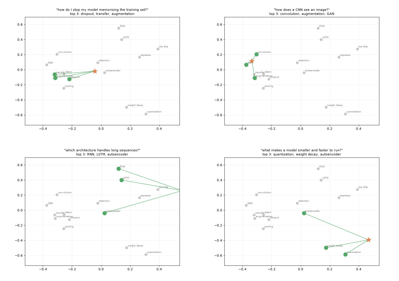Each query lands in the same space as the documents; retrieval is just its nearest neighbours.

6. Chunking¶

Real documents are far longer than these one-line examples, and that creates two problems:

1. The encoder has a token limit (512 for this model, and it was trained on much shorter text). Anything past it is silently truncated.
2. One vector cannot represent ten paragraphs. Averaging a whole page produces a vague vector that matches everything weakly and nothing strongly.

So we split documents into chunks and embed each one. Chunk size is a genuine trade-off:

Chunk size	Retrieval precision	Context for the answer
Too small (a sentence)	sharp — matches exactly	may not contain the whole answer
Too large (a page)	vague — diluted vectors	plenty, but mostly irrelevant filler

Overlap between consecutive chunks is the standard mitigation: it stops an answer that straddles a boundary from being cut in half.

In [13]:

def chunk_text(text, chunk_words=40, overlap=10):
    """Split into word windows with overlap, so answers spanning a boundary survive."""
    words = text.split()
    step = max(chunk_words - overlap, 1)
    chunks = []
    for start in range(0, max(len(words) - overlap, 1), step):
        chunk = words[start:start + chunk_words]
        if chunk:
            chunks.append(' '.join(chunk))
        if start + chunk_words >= len(words):
            break
    return chunks

DOCUMENT = """
Regularization is the collective name for techniques that improve how well a network
generalises to unseen data. The most common is dropout, which randomly switches off a
fraction of the units on every forward pass, so the network cannot become dependent on
any single neuron. Weight decay takes a different approach and adds the squared norm of
the parameters to the loss, which keeps the weights small and the decision boundary
smooth. Batch normalization standardises each layer's inputs across the batch, which
mainly speeds up convergence but also regularises mildly. Data augmentation is usually
the most effective option for images, because it multiplies the effective size of the
training set at no cost in model capacity. Finally, early stopping simply halts training
when the validation loss stops improving, and restores the best weights seen so far.
""".strip()

for size, overlap in [(20, 5), (40, 10), (200, 20)]:
    chunks = chunk_text(DOCUMENT, size, overlap)
    print(f'chunk_words={size:3d}, overlap={overlap:2d}  ->  {len(chunks)} chunks, '
          f'first is {len(chunks[0].split())} words')

chunks = chunk_text(DOCUMENT, 40, 10)
print('\nFirst chunk:\n ', chunks[0][:150], '...')
print('\nSecond chunk (note the repeated words at the start):\n ', chunks[1][:150], '...')

def chunk_text(text, chunk_words=40, overlap=10): """Split into word windows with overlap, so answers spanning a boundary survive.""" words = text.split() step = max(chunk_words - overlap, 1) chunks = [] for start in range(0, max(len(words) - overlap, 1), step): chunk = words[start:start + chunk_words] if chunk: chunks.append(' '.join(chunk)) if start + chunk_words >= len(words): break return chunks DOCUMENT = """ Regularization is the collective name for techniques that improve how well a network generalises to unseen data. The most common is dropout, which randomly switches off a fraction of the units on every forward pass, so the network cannot become dependent on any single neuron. Weight decay takes a different approach and adds the squared norm of the parameters to the loss, which keeps the weights small and the decision boundary smooth. Batch normalization standardises each layer's inputs across the batch, which mainly speeds up convergence but also regularises mildly. Data augmentation is usually the most effective option for images, because it multiplies the effective size of the training set at no cost in model capacity. Finally, early stopping simply halts training when the validation loss stops improving, and restores the best weights seen so far. """.strip() for size, overlap in [(20, 5), (40, 10), (200, 20)]: chunks = chunk_text(DOCUMENT, size, overlap) print(f'chunk_words={size:3d}, overlap={overlap:2d} -> {len(chunks)} chunks, ' f'first is {len(chunks[0].split())} words') chunks = chunk_text(DOCUMENT, 40, 10) print('\nFirst chunk:\n ', chunks[0][:150], '...') print('\nSecond chunk (note the repeated words at the start):\n ', chunks[1][:150], '...')

chunk_words= 20, overlap= 5  ->  9 chunks, first is 20 words
chunk_words= 40, overlap=10  ->  5 chunks, first is 40 words
chunk_words=200, overlap=20  ->  1 chunks, first is 136 words

First chunk:
  Regularization is the collective name for techniques that improve how well a network generalises to unseen data. The most common is dropout, which ran ...

Second chunk (note the repeated words at the start):
  units on every forward pass, so the network cannot become dependent on any single neuron. Weight decay takes a different approach and adds the squared ...

In [14]:

# Which chunk answers a specific question?
chunk_vectors = embed(chunks)
for query in ['what does weight decay do to the weights?',
              'when should I stop training?']:
    best, score = search(query, chunk_vectors, chunks, k=1)[0]
    print(f'\n"{query}"  ({score:.3f})\n   {best[:170]}...')

# Which chunk answers a specific question? chunk_vectors = embed(chunks) for query in ['what does weight decay do to the weights?', 'when should I stop training?']: best, score = search(query, chunk_vectors, chunks, k=1)[0] print(f'\n"{query}" ({score:.3f})\n {best[:170]}...')

"what does weight decay do to the weights?"  (0.605)
   units on every forward pass, so the network cannot become dependent on any single neuron. Weight decay takes a different approach and adds the squared norm of the paramet...

"when should I stop training?"  (0.467)
   halts training when the validation loss stops improving, and restores the best weights seen so far....

7. Measuring Retrieval Quality¶

"It looks about right" is not an evaluation. The two standard metrics are cheap to compute and worth having before you tune anything:

• Recall@k — the fraction of queries whose correct document appears in the top $k$. This is what matters for RAG: if the right passage is not retrieved, the generator cannot possibly answer.
• MRR (Mean Reciprocal Rank) — the average of $1/\text{rank}$ of the first correct hit. It rewards putting the right answer first, not merely somewhere in the list.

In [15]:

# Query -> index of the document that should be retrieved
EVAL_SET = [
    ('how do I stop my model memorising the training set?', 0),
    ('what keeps the weights small?', 1),
    ('how can I get more training images for free?', 2),
    ('how does a filter move across an image?', 3),
    ('how do I make feature maps smaller?', 4),
    ('which model remembers things across many time steps?', 5),
    ('how does a model look at every position at once?', 7),
    ('how do I reuse a pretrained network?', 8),
    ('how do I shrink a model for deployment?', 11),
    ('which optimizer adapts its step size per parameter?', 12),
]

def evaluate_retrieval(eval_set, vectors, k_values=(1, 3, 5)):
    query_vecs = embed([q for q, _ in eval_set])
    scores = query_vecs @ vectors.T                     # (queries, documents)
    ranking = scores.argsort(dim=1, descending=True)

    ranks = []
    for row, (_, gold) in zip(ranking, eval_set):
        ranks.append((row == gold).nonzero()[0, 0].item() + 1)   # 1-based rank
    ranks = np.array(ranks)

    results = {f'recall@{k}': float((ranks <= k).mean()) for k in k_values}
    results['MRR'] = float((1 / ranks).mean())
    return results, ranks

results, ranks = evaluate_retrieval(EVAL_SET, corpus_vectors)
for name, value in results.items():
    print(f'{name:10s} {value:.3f}')
print('\nRank of the correct document, per query:')
for (query, _), rank in zip(EVAL_SET, ranks):
    flag = '' if rank == 1 else '   <-- not first'
    print(f'  rank {rank}  "{query[:52]}"{flag}')

# Query -> index of the document that should be retrieved EVAL_SET = [ ('how do I stop my model memorising the training set?', 0), ('what keeps the weights small?', 1), ('how can I get more training images for free?', 2), ('how does a filter move across an image?', 3), ('how do I make feature maps smaller?', 4), ('which model remembers things across many time steps?', 5), ('how does a model look at every position at once?', 7), ('how do I reuse a pretrained network?', 8), ('how do I shrink a model for deployment?', 11), ('which optimizer adapts its step size per parameter?', 12), ] def evaluate_retrieval(eval_set, vectors, k_values=(1, 3, 5)): query_vecs = embed([q for q, _ in eval_set]) scores = query_vecs @ vectors.T # (queries, documents) ranking = scores.argsort(dim=1, descending=True) ranks = [] for row, (_, gold) in zip(ranking, eval_set): ranks.append((row == gold).nonzero()[0, 0].item() + 1) # 1-based rank ranks = np.array(ranks) results = {f'recall@{k}': float((ranks <= k).mean()) for k in k_values} results['MRR'] = float((1 / ranks).mean()) return results, ranks results, ranks = evaluate_retrieval(EVAL_SET, corpus_vectors) for name, value in results.items(): print(f'{name:10s} {value:.3f}') print('\nRank of the correct document, per query:') for (query, _), rank in zip(EVAL_SET, ranks): flag = '' if rank == 1 else ' <-- not first' print(f' rank {rank} "{query[:52]}"{flag}')

recall@1   0.700
recall@3   1.000
recall@5   1.000
MRR        0.850

Rank of the correct document, per query:
  rank 1  "how do I stop my model memorising the training set?"
  rank 1  "what keeps the weights small?"
  rank 2  "how can I get more training images for free?"   <-- not first
  rank 1  "how does a filter move across an image?"
  rank 1  "how do I make feature maps smaller?"
  rank 1  "which model remembers things across many time steps?"
  rank 2  "how does a model look at every position at once?"   <-- not first
  rank 1  "how do I reuse a pretrained network?"
  rank 2  "how do I shrink a model for deployment?"   <-- not first
  rank 1  "which optimizer adapts its step size per parameter?"

In [16]:

# The keyword baseline, scored the same way
keyword_ranks = []
for query, gold in EVAL_SET:
    scored = sorted(range(len(CORPUS)),
                    key=lambda i: keyword_score(query, CORPUS[i]), reverse=True)
    keyword_ranks.append(scored.index(gold) + 1)
keyword_ranks = np.array(keyword_ranks)

fig, ax = plt.subplots(figsize=(8, 4))
x = np.arange(len(EVAL_SET))
ax.bar(x - 0.2, keyword_ranks, width=0.4, label='word overlap', color='#C44E52')
ax.bar(x + 0.2, ranks, width=0.4, label='embeddings', color='#4C72B0')
ax.axhline(1, color='gray', linestyle=':', label='perfect (rank 1)')
ax.set_xticks(x, [q[:16] + '...' for q, _ in EVAL_SET], rotation=45, ha='right', fontsize=8)
ax.set_ylabel('rank of the correct document (lower is better)')
ax.set_title('Embeddings vs keyword matching')
ax.legend()
plt.tight_layout()
plt.show()

print(f'Keyword   MRR: {(1 / keyword_ranks).mean():.3f},  recall@1: {(keyword_ranks == 1).mean():.2f}')
print(f'Embedding MRR: {(1 / ranks).mean():.3f},  recall@1: {(ranks == 1).mean():.2f}')

# The keyword baseline, scored the same way keyword_ranks = [] for query, gold in EVAL_SET: scored = sorted(range(len(CORPUS)), key=lambda i: keyword_score(query, CORPUS[i]), reverse=True) keyword_ranks.append(scored.index(gold) + 1) keyword_ranks = np.array(keyword_ranks) fig, ax = plt.subplots(figsize=(8, 4)) x = np.arange(len(EVAL_SET)) ax.bar(x - 0.2, keyword_ranks, width=0.4, label='word overlap', color='#C44E52') ax.bar(x + 0.2, ranks, width=0.4, label='embeddings', color='#4C72B0') ax.axhline(1, color='gray', linestyle=':', label='perfect (rank 1)') ax.set_xticks(x, [q[:16] + '...' for q, _ in EVAL_SET], rotation=45, ha='right', fontsize=8) ax.set_ylabel('rank of the correct document (lower is better)') ax.set_title('Embeddings vs keyword matching') ax.legend() plt.tight_layout() plt.show() print(f'Keyword MRR: {(1 / keyword_ranks).mean():.3f}, recall@1: {(keyword_ranks == 1).mean():.2f}') print(f'Embedding MRR: {(1 / ranks).mean():.3f}, recall@1: {(ranks == 1).mean():.2f}')

Keyword   MRR: 0.616,  recall@1: 0.50
Embedding MRR: 0.850,  recall@1: 0.70

Hybrid search. Embeddings are not strictly better. Keyword matching still wins on exact identifiers — product codes, error numbers, surnames — where the "meaning" of a token is that exact string. Production systems usually run both and fuse the rankings, which beats either alone.

8. Scaling the Index¶

Our search is a brute-force matrix multiply: exact, and $O(n)$ in the corpus size. That is genuinely fine up to a surprisingly large number of vectors. Beyond that, approximate nearest neighbour (ANN) indexes — FAISS, HNSW, ScaNN — trade a little recall for logarithmic search time.

Let's measure where brute force starts to hurt, on this machine.

In [17]:

dim = corpus_vectors.shape[1]
sizes = [1_000, 10_000, 100_000, 500_000]
timings = []

query = embed('how do I stop my model memorising the training set?')
for n in sizes:
    fake_index = F.normalize(torch.randn(n, dim), p=2, dim=1)
    t0 = time.perf_counter()
    for _ in range(5):
        (fake_index @ query.T).squeeze(1).topk(5)
    timings.append((time.perf_counter() - t0) / 5 * 1000)
    del fake_index

fig, ax = plt.subplots(figsize=(7, 4))
ax.plot(sizes, timings, marker='o')
ax.set_xscale('log'); ax.set_yscale('log')
ax.set_xlabel('vectors in the index'); ax.set_ylabel('exact search time (ms)')
ax.set_title('Brute-force search scales linearly')
ax.grid(alpha=0.3, which='both')
plt.tight_layout()
plt.show()

for n, ms in zip(sizes, timings):
    print(f'{n:>8,} vectors: {ms:7.2f} ms   ({n * dim * 4 / 1e6:.0f} MB of float32)')
print('\nBelow ~100k vectors, brute force is simpler, exact, and fast enough.')
print('Above that, reach for an ANN index - and measure the recall you gave up.')

dim = corpus_vectors.shape[1] sizes = [1_000, 10_000, 100_000, 500_000] timings = [] query = embed('how do I stop my model memorising the training set?') for n in sizes: fake_index = F.normalize(torch.randn(n, dim), p=2, dim=1) t0 = time.perf_counter() for _ in range(5): (fake_index @ query.T).squeeze(1).topk(5) timings.append((time.perf_counter() - t0) / 5 * 1000) del fake_index fig, ax = plt.subplots(figsize=(7, 4)) ax.plot(sizes, timings, marker='o') ax.set_xscale('log'); ax.set_yscale('log') ax.set_xlabel('vectors in the index'); ax.set_ylabel('exact search time (ms)') ax.set_title('Brute-force search scales linearly') ax.grid(alpha=0.3, which='both') plt.tight_layout() plt.show() for n, ms in zip(sizes, timings): print(f'{n:>8,} vectors: {ms:7.2f} ms ({n * dim * 4 / 1e6:.0f} MB of float32)') print('\nBelow ~100k vectors, brute force is simpler, exact, and fast enough.') print('Above that, reach for an ANN index - and measure the recall you gave up.')

   1,000 vectors:    0.21 ms   (2 MB of float32)
  10,000 vectors:    0.84 ms   (15 MB of float32)
 100,000 vectors:    8.97 ms   (154 MB of float32)
 500,000 vectors:   33.68 ms   (768 MB of float32)

Below ~100k vectors, brute force is simpler, exact, and fast enough.
Above that, reach for an ANN index - and measure the recall you gave up.

9. Experiment: Try Different Settings¶

You can experiment with:

• Turning off normalize in embed and seeing how the rankings change once length affects the score
• Replacing mean pooling with CLS pooling (hidden[:, 0]) — this model was not trained for it, and the quality drop is instructive
• Swapping in a larger encoder such as sentence-transformers/all-mpnet-base-v2 and re-running the evaluation
• Adding your own documents and queries to EVAL_SET, then tuning chunk size against recall@k
• Building an index over a real text file — a README, a book, your own notes
• Implementing hybrid search: normalise the keyword and embedding scores, and combine them with a weight
• Trying faiss-cpu and measuring both the speedup and the recall you lost

Try modifying the code above and observe how the retrieval quality changes.

10. Conclusion¶

In this lab, you turned a pretrained Transformer into a search engine. Mean pooling collapses per-token vectors into one sentence vector, normalisation makes the dot product a cosine similarity, and the whole search becomes a single matrix multiplication.

Key takeaways:

• Embeddings match meaning; keywords match strings. Both have cases where they win.
• Mean pool with the attention mask, and normalise — then similarity is just a dot product.
• Chunk size is a real trade-off between retrieval precision and having enough context.
• A vector search always returns something. If you need "no answer", you must threshold.
• Measure with recall@k and MRR before tuning anything, and keep a keyword baseline honest.
• Brute force is fine for small corpora; ANN indexes trade recall for speed at scale.

The next lab feeds these retrieved passages to a language model, which is where retrieval turns into answers.