Lab 10: Recurrent Neural Networks (RNN)
In this lab, you will learn about Recurrent Neural Networks (RNNs), the family of models designed to work with sequential data such as time series, text, audio, and sensor readings. You will build an RNN cell by hand, use PyTorch's built-in nn.RNN, and train a network to forecast a signal.
We will cover the following topics:
- Why dense and convolutional networks struggle with sequences
- The RNN cell: hidden state, recurrence, and parameter sharing
- Implementing an RNN cell from scratch and checking it against PyTorch
- Building and training an RNN for time-series forecasting
- The vanishing gradient problem and why it motivates LSTMs
1. Why Sequences Need a Different Model
The networks you built in the previous labs make one strong assumption: every input has a fixed size, and the order of the samples does not matter. A dense network for the make_moons dataset (Lab 08) sees two numbers. A CNN for MNIST (Lab 09) sees a 28x28 grid.
Sequential data breaks both assumptions:
- Variable length: one sentence has 5 words, the next has 40. One patient's ECG is 3 seconds long, another's is 30.
- Order carries meaning: "the dog bit the man" and "the man bit the dog" contain the same words in a different order, and mean different things.
- Context matters: to predict tomorrow's temperature you need what happened over the past days, not just today.
You could flatten a sequence and feed it to a dense network, but then:
- The network only accepts sequences of exactly the length you trained on.
- A pattern learned at position 3 has to be re-learned from scratch at position 17, because the weights that read those positions are different.
An RNN solves both problems by processing the sequence one step at a time while carrying a memory of everything it has seen so far.
2. What is a Recurrent Neural Network?
A Recurrent Neural Network processes a sequence $x_1, x_2, \ldots, x_T$ one element at a time. At every step it keeps a hidden state $h_t$ — a vector that summarises the sequence so far — and updates it using the current input and the previous hidden state.
The crucial idea is that the same weights are reused at every time step. The network is a small function applied over and over, not a large function applied once. Drawing the same cell repeated across time is called unrolling the network.
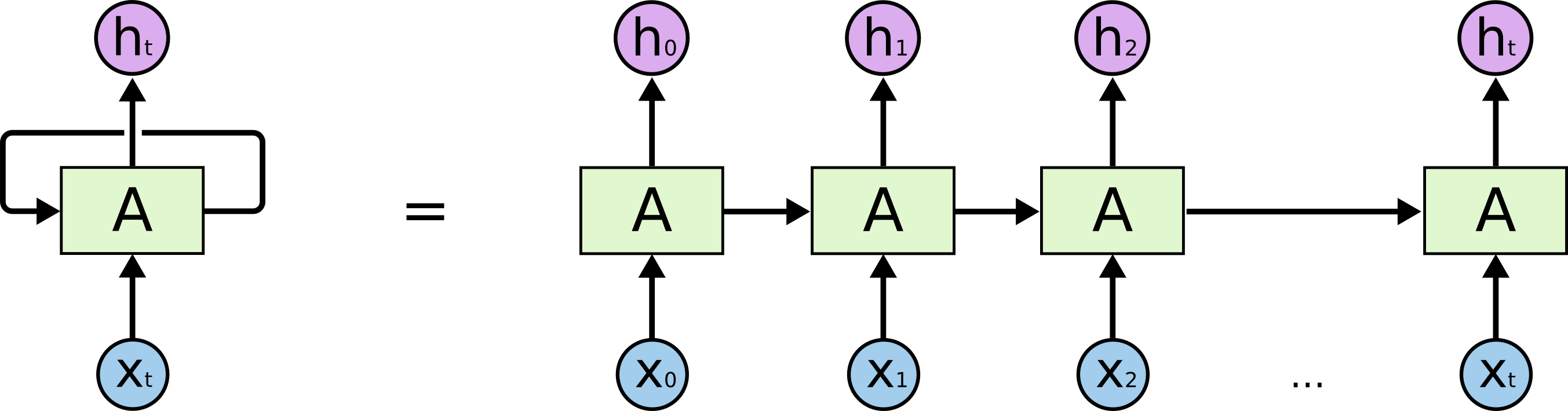 An RNN unrolled through time. The same cell (same weights) is applied at every step, passing a hidden state forward.
Source: colah.github.io
Key characteristics:
- Hidden state: a running summary of the sequence, updated at each step.
- Parameter sharing: one set of weights handles a sequence of any length.
- Directional: information flows from earlier steps to later ones.
Zooming in on a single step, the cell takes two things in — the current input and the previous memory — mixes them with one weight matrix each, and squashes the result:

3. The RNN Cell, Step by Step
At each time step $t$, a vanilla ("Elman") RNN computes:
$$ h_t = \tanh\left(W_{ih}\,x_t + b_{ih} + W_{hh}\,h_{t-1} + b_{hh}\right) $$
and the output at that step is a linear read-out of the hidden state:
$$ y_t = W_{ho}\,h_t + b_{ho} $$
where:
- $x_t \in \mathbb{R}^{n_{in}}$ is the input at step $t$
- $h_t \in \mathbb{R}^{n_{h}}$ is the hidden state, with $h_0$ usually initialised to zeros
- $W_{ih} \in \mathbb{R}^{n_h \times n_{in}}$ maps the input into hidden space
- $W_{hh} \in \mathbb{R}^{n_h \times n_h}$ maps the previous hidden state into hidden space
- $\tanh$ squashes the result into $(-1, 1)$, keeping the state bounded
Notice there is no index $t$ on the weights: $W_{ih}$, $W_{hh}$, $b_{ih}$ and $b_{hh}$ are the same matrices at every step. That is what parameter sharing means in practice.
Implementing an RNN cell from scratch
Let's write the recurrence ourselves with plain tensor operations, then check that PyTorch's nn.RNNCell produces exactly the same numbers when given the same weights.
import torch
import torch.nn as nn

torch.manual_seed(0)

input_size = 3    # number of features per time step
hidden_size = 4   # size of the memory vector
seq_len = 5       # number of time steps

# One sequence: (seq_len, input_size)
x_seq = torch.randn(seq_len, input_size)

# PyTorch's own cell, so we can borrow its weights
cell = nn.RNNCell(input_size, hidden_size, nonlinearity='tanh')

def manual_rnn_cell(x_t, h_prev, cell):
    """One RNN step written out by hand: h_t = tanh(W_ih x_t + b_ih + W_hh h_{t-1} + b_hh)."""
    return torch.tanh(
        x_t @ cell.weight_ih.T + cell.bias_ih
        + h_prev @ cell.weight_hh.T + cell.bias_hh
    )

# Run the recurrence manually over the sequence
h_manual = torch.zeros(1, hidden_size)   # h_0
manual_states = []
for t in range(seq_len):
    h_manual = manual_rnn_cell(x_seq[t].unsqueeze(0), h_manual, cell)
    manual_states.append(h_manual)

# Run the same sequence through PyTorch's cell
h_torch = torch.zeros(1, hidden_size)
torch_states = []
for t in range(seq_len):
    h_torch = cell(x_seq[t].unsqueeze(0), h_torch)
    torch_states.append(h_torch)

print('Manual  h_T:', manual_states[-1].detach().numpy().round(4))
print('PyTorch h_T:', torch_states[-1].detach().numpy().round(4))
print('Match:', torch.allclose(manual_states[-1], torch_states[-1], atol=1e-6))
Manual  h_T: [[ 0.3659 -0.4076 -0.3544  0.7706]]
PyTorch h_T: [[ 0.3659 -0.4076 -0.3544  0.7706]]
Match: True
Watching the hidden state evolve
The hidden state is just a vector of numbers that changes as the sequence is consumed. Animating it makes the "memory" concrete: each bar is one memory slot, and you can watch the whole vector get rewritten at every step.
import matplotlib.pyplot as plt
from matplotlib import animation
import os

os.makedirs('Misc', exist_ok=True)

def save_animation(ani, filename, fps=8, dpi=80):
    """Render an animation to a GIF under Misc/ and report where it went."""
    path = os.path.join('Misc', filename)
    ani.save(path, writer='pillow', fps=fps, dpi=dpi)
    print(f'saved {path}  ({os.path.getsize(path) / 1e6:.1f} MB)')
    return path

states = torch.cat(manual_states).detach().numpy()   # (seq_len, hidden_size)

fig, (ax_in, ax_h) = plt.subplots(1, 2, figsize=(9, 3.2), gridspec_kw={'width_ratios': [1, 1.4]})

ax_in.set_title('input $x_t$')
ax_in.set_ylim(-3, 3)
ax_in.set_xticks(range(input_size))
ax_in.axhline(0, color='gray', lw=0.8)
in_bars = ax_in.bar(range(input_size), [0] * input_size, color='#64B5CD')

ax_h.set_title('hidden state $h_t$')
ax_h.set_ylim(-1.05, 1.05)
ax_h.set_xticks(range(hidden_size))
ax_h.set_xlabel('memory slot')
ax_h.axhline(0, color='gray', lw=0.8)
h_bars = ax_h.bar(range(hidden_size), [0] * hidden_size, color='#8172B3')

def update(t):
    for bar, v in zip(in_bars, x_seq[t].numpy()):
        bar.set_height(v)
    for bar, v in zip(h_bars, states[t]):
        bar.set_height(v)
    fig.suptitle(f'time step t = {t + 1} of {seq_len}')
    return list(in_bars) + list(h_bars)

ani = animation.FuncAnimation(fig, update, frames=seq_len, interval=900, blit=False)
plt.close(fig)   # stop the final frame from also being drawn as a static image
save_animation(ani, 'lab10_hidden_state.gif', fps=2)
saved Misc\lab10_hidden_state.gif (0.0 MB)
'Misc\\lab10_hidden_state.gif'
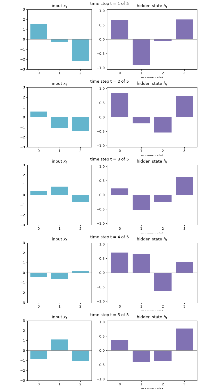 The hidden state is completely rewritten at every time step.
4. RNNs in PyTorch: nn.RNN
Looping over time steps by hand is instructive but slow. nn.RNN runs the whole loop for you in optimised code.
The shape conventions are the part that trips people up, so it is worth stating them once:
- Input with
batch_first=True:(batch_size, seq_len, input_size) - Initial hidden state
h0:(num_layers, batch_size, hidden_size)— note this is not batch-first, even whenbatch_first=True - Output
out:(batch_size, seq_len, hidden_size)— the hidden state at every time step - Final hidden state
hn:(num_layers, batch_size, hidden_size)— the state after the last step
For a forecasting or classification task you usually only need the last step, out[:, -1, :]. For tagging every element of a sequence you need all of out.
# Import PyTorch and check version
import torch
import torch.nn as nn
import torch.optim as optim
print('PyTorch version:', torch.__version__)

# A batch of 2 sequences, 5 time steps each, 3 features per step
batch = torch.randn(2, 5, 3)

rnn = nn.RNN(input_size=3, hidden_size=4, num_layers=1, batch_first=True)
out, hn = rnn(batch)

print('input shape :', tuple(batch.shape))
print('out shape   :', tuple(out.shape), '<- hidden state at every time step')
print('hn shape    :', tuple(hn.shape), '<- hidden state after the last step')

# The last column of `out` is the same thing as `hn` for a single-layer RNN
print('out[:, -1, :] == hn[-1]:', torch.allclose(out[:, -1, :], hn[-1]))
PyTorch version: 2.13.0+cpu
input shape : (2, 5, 3)
out shape   : (2, 5, 4) <- hidden state at every time step
hn shape    : (1, 2, 4) <- hidden state after the last step
out[:, -1, :] == hn[-1]: True
5. Dataset Preparation
We will forecast a noisy periodic signal — the "hello world" of sequence modelling. The task is: given the last 20 values, predict the next one.
To turn a single long series into a supervised dataset we slide a window across it. Each window of length seq_len becomes an input, and the value immediately after the window becomes the target.
An important detail: because the data is a time series, we split it chronologically rather than randomly. Shuffling before splitting would let the model peek at the future, and the test score would be meaningless.

import numpy as np

# Generate a noisy signal: a sine wave with a second, slower component
np.random.seed(42)
n_points = 1500
t = np.linspace(0, 60, n_points)
series = np.sin(t) + 0.5 * np.sin(0.3 * t) + 0.02 * np.random.randn(n_points)

plt.figure(figsize=(10, 3))
plt.plot(t[:400], series[:400])
plt.title('The signal we will forecast (first 400 points)')
plt.xlabel('t')
plt.ylabel('value')
plt.grid(alpha=0.3)
plt.show()

def make_windows(series, seq_len):
    """Slide a window over a 1-D series to build (input, target) pairs."""
    X, y = [], []
    for i in range(len(series) - seq_len):
        X.append(series[i:i + seq_len])
        y.append(series[i + seq_len])
    X = np.array(X, dtype=np.float32)
    y = np.array(y, dtype=np.float32)
    return X, y

seq_len = 20
X, y = make_windows(series, seq_len)

# Chronological split: the first 80% for training, the rest for testing
split = int(0.8 * len(X))
X_train, X_test = X[:split], X[split:]
y_train, y_test = y[:split], y[split:]

# RNNs expect (batch, seq_len, input_size); our signal has 1 feature per step
X_train = torch.tensor(X_train).unsqueeze(-1)
X_test = torch.tensor(X_test).unsqueeze(-1)
y_train = torch.tensor(y_train).unsqueeze(-1)
y_test = torch.tensor(y_test).unsqueeze(-1)

print('X_train:', tuple(X_train.shape), ' y_train:', tuple(y_train.shape))
print('X_test :', tuple(X_test.shape), ' y_test :', tuple(y_test.shape))
X_train: (1184, 20, 1)  y_train: (1184, 1)
X_test : (296, 20, 1)  y_test : (296, 1)
from torch.utils.data import TensorDataset, DataLoader

train_loader = DataLoader(TensorDataset(X_train, y_train), batch_size=32, shuffle=True)
test_loader = DataLoader(TensorDataset(X_test, y_test), batch_size=256, shuffle=False)
6. Defining an RNN in PyTorch
The model is small: an nn.RNN to consume the window, then a nn.Linear to turn the final hidden state into a single predicted number.
Shuffling the windows during training is fine, by the way — the order inside each window is what carries the temporal information, and that stays intact.
class SimpleRNN(nn.Module):
    def __init__(self, input_size=1, hidden_size=32, num_layers=1, output_size=1):
        super(SimpleRNN, self).__init__()
        self.hidden_size = hidden_size
        self.num_layers = num_layers
        self.rnn = nn.RNN(input_size, hidden_size, num_layers, batch_first=True)
        self.fc = nn.Linear(hidden_size, output_size)

    def forward(self, x):
        # h0 defaults to zeros if we do not pass it, but being explicit is clearer
        h0 = torch.zeros(self.num_layers, x.size(0), self.hidden_size, device=x.device)
        out, hn = self.rnn(x, h0)     # out: (batch, seq_len, hidden_size)
        last = out[:, -1, :]          # keep only the final time step
        return self.fc(last)

model = SimpleRNN()
print(model)
print('Trainable parameters:', sum(p.numel() for p in model.parameters() if p.requires_grad))
SimpleRNN(
  (rnn): RNN(1, 32, batch_first=True)
  (fc): Linear(in_features=32, out_features=1, bias=True)
)
Trainable parameters: 1153
7. Training the RNN
Forecasting a continuous value is a regression problem, so we use mean squared error (nn.MSELoss) together with the Adam optimizer — the same recipe as Lab 08, only the model changed.
device = torch.device('cuda' if torch.cuda.is_available() else 'cpu')
model.to(device)

criterion = nn.MSELoss()
optimizer = optim.Adam(model.parameters(), lr=0.01)

num_epochs = 20
train_losses, test_losses = [], []

for epoch in range(num_epochs):
    model.train()
    running = 0.0
    for xb, yb in train_loader:
        xb, yb = xb.to(device), yb.to(device)
        optimizer.zero_grad()
        pred = model(xb)
        loss = criterion(pred, yb)
        loss.backward()
        optimizer.step()
        running += loss.item() * xb.size(0)
    train_losses.append(running / len(train_loader.dataset))

    model.eval()
    running = 0.0
    with torch.no_grad():
        for xb, yb in test_loader:
            xb, yb = xb.to(device), yb.to(device)
            running += criterion(model(xb), yb).item() * xb.size(0)
    test_losses.append(running / len(test_loader.dataset))

    if (epoch + 1) % 5 == 0:
        print(f'Epoch [{epoch+1}/{num_epochs}], '
              f'Train MSE: {train_losses[-1]:.5f}, Test MSE: {test_losses[-1]:.5f}')
Epoch [5/20], Train MSE: 0.00137, Test MSE: 0.00126
Epoch [10/20], Train MSE: 0.00125, Test MSE: 0.00135
Epoch [15/20], Train MSE: 0.00112, Test MSE: 0.00087
Epoch [20/20], Train MSE: 0.00103, Test MSE: 0.00109
plt.figure(figsize=(6, 4))
plt.plot(train_losses, label='train')
plt.plot(test_losses, label='test')
plt.xlabel('Epoch')
plt.ylabel('MSE loss')
plt.title('Training Loss Curve')
plt.legend()
plt.grid(alpha=0.3)
plt.show()

8. Evaluating the Model
There are two very different ways to evaluate a forecaster, and confusing them is a classic mistake.
One-step-ahead prediction: at every point, feed the model the true last 20 values and ask for the next one. This is what the model was trained to do, and it is what the loss above measures.
model.eval()
with torch.no_grad():
    preds = model(X_test.to(device)).cpu().numpy().ravel()

truth = y_test.numpy().ravel()
rmse = np.sqrt(((preds - truth) ** 2).mean())
# A baseline worth beating: "tomorrow looks like today"
naive = X_test[:, -1, 0].numpy()
naive_rmse = np.sqrt(((naive - truth) ** 2).mean())

print(f'RNN   RMSE: {rmse:.4f}')
print(f'Naive RMSE: {naive_rmse:.4f}  (predict the last observed value)')
print(f'The RNN is {naive_rmse / rmse:.1f}x better than the baseline.')
print('\nAlways print this comparison. On a smooth, slowly-changing series the naive')
print('baseline is very hard to beat, and a model that loses to it has learned nothing.')

plt.figure(figsize=(10, 3))
plt.plot(truth[:200], label='actual')
plt.plot(preds[:200], label='predicted', linestyle='--')
plt.title('One-step-ahead predictions on the test set')
plt.xlabel('test time step')
plt.legend()
plt.grid(alpha=0.3)
plt.show()
RNN   RMSE: 0.0330
Naive RMSE: 0.0395  (predict the last observed value)
The RNN is 1.2x better than the baseline.

Always print this comparison. On a smooth, slowly-changing series the naive
baseline is very hard to beat, and a model that loses to it has learned nothing.

Free-running (multi-step) generation: start from one real window, then keep feeding the model its own predictions. Nothing corrects it along the way, so small errors compound. This is a much harder test, and it shows how far ahead the model is actually useful.
model.eval()
window = X_test[0].clone().to(device)   # (seq_len, 1) — one real window to start from
generated = []
horizon = 100

with torch.no_grad():
    for _ in range(horizon):
        nxt = model(window.unsqueeze(0))          # (1, 1)
        generated.append(nxt.item())
        # drop the oldest step, append the prediction as the newest
        window = torch.cat([window[1:], nxt.view(1, 1)], dim=0)

fig, ax = plt.subplots(figsize=(9, 3.2))
ax.plot(truth[:horizon], color='#4C72B0', label='actual')
line, = ax.plot([], [], color='#DD8452', linestyle='--', label='free-running forecast')
head, = ax.plot([], [], 'o', color='#DD8452')
ax.set_xlim(0, horizon - 1)
ax.set_ylim(min(min(generated), truth[:horizon].min()) - 0.3,
            max(max(generated), truth[:horizon].max()) + 0.3)
ax.set_xlabel('steps ahead')
ax.legend(loc='upper right')
ax.grid(alpha=0.3)

def update(k):
    line.set_data(range(k + 1), generated[:k + 1])
    head.set_data([k], [generated[k]])
    ax.set_title(f'Feeding predictions back in: step {k + 1} of {horizon}')
    return line, head

ani = animation.FuncAnimation(fig, update, frames=horizon, interval=60, blit=False)
plt.close(fig)
save_animation(ani, 'lab10_free_running.gif', fps=12)
saved Misc\lab10_free_running.gif (0.3 MB)
'Misc\\lab10_free_running.gif'
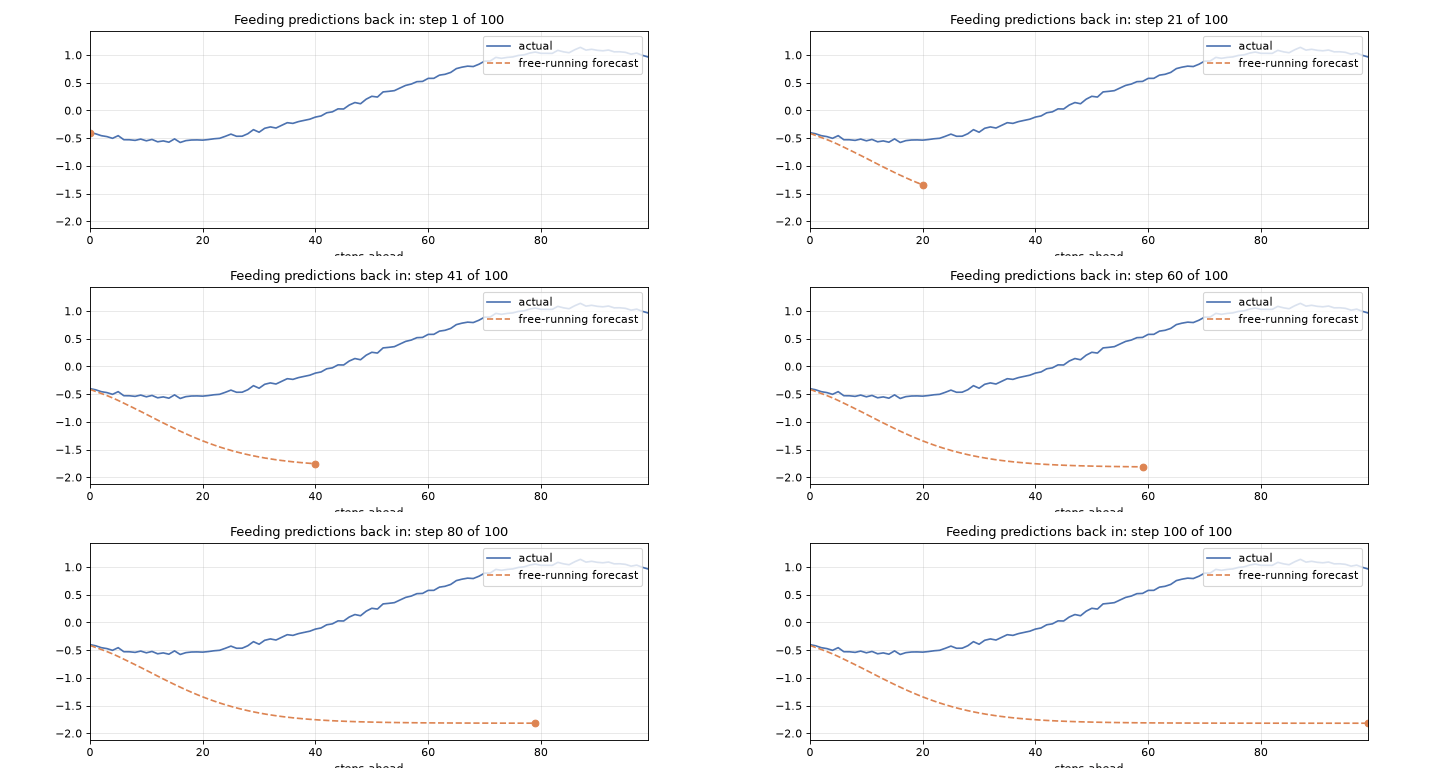 Free-running forecast: the model is fed its own predictions, and the error compounds.
Watch where the dashed line stops tracking the solid one. Up to that point the model is genuinely useful; past it, it is drifting on its own errors. That crossover — not the training loss — is the number to quote when someone asks "how far ahead can this thing predict?"
9. The Vanishing Gradient Problem
Vanilla RNNs have a well-known weakness: they forget. Training uses backpropagation through time, which unrolls the network and applies the chain rule backwards across every step. The gradient reaching step $t$ from step $T$ contains a product of $T - t$ Jacobians:
$$ \frac{\partial h_T}{\partial h_t} = \prod_{k=t+1}^{T} \frac{\partial h_k}{\partial h_{k-1}} $$
Each factor involves $W_{hh}$ and the derivative of $\tanh$, which is at most 1 and usually much smaller. Multiplying many such terms drives the product towards zero: the vanishing gradient problem. (When the weights are large the opposite happens and the product explodes, which is why gradient clipping is standard practice for RNNs.)
The practical consequence: a vanilla RNN learns short-range patterns well and long-range ones barely at all.
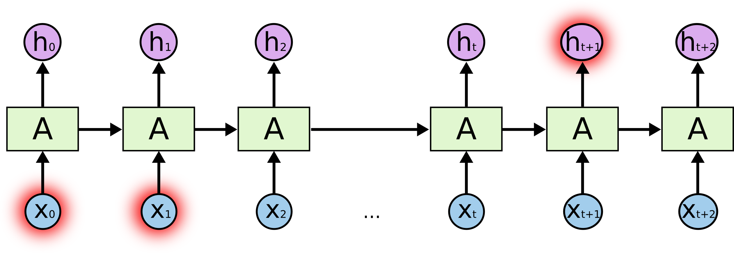 When the relevant context is far in the past, the gradient signal connecting it to the output has faded away.
Source: colah.github.io
Let's measure it. We push a sequence of length $T$ through an RNN and ask: how strongly does the first input influence the final hidden state?
def gradient_reaching_first_step(T, hidden_size=32):
    """Norm of d(sum of h_T) / d(x_1) for a sequence of length T."""
    torch.manual_seed(0)
    probe = nn.RNN(input_size=1, hidden_size=hidden_size, batch_first=True)
    x = torch.randn(1, T, 1, requires_grad=True)
    out, _ = probe(x)
    out[:, -1, :].sum().backward()
    return x.grad[0, 0].norm().item()

print(f'{"seq length":>12} | {"gradient at first step":>22}')
print('-' * 38)
for T in [5, 10, 20, 40, 80, 160]:
    print(f'{T:>12} | {gradient_reaching_first_step(T):>22.3e}')
  seq length | gradient at first step
--------------------------------------
           5 |              5.518e-02
          10 |              5.026e-03
          20 |              3.673e-05
          40 |              1.750e-09
          80 |              4.265e-18
         160 |              5.279e-36
The gradient shrinks by orders of magnitude as the sequence grows. By 80 or 160 steps the first input has essentially no influence on the loss, so the network cannot learn anything that depends on it.
This is exactly the problem LSTM networks were invented to solve, and that is the subject of Lab 11.
10. Experiment: Try Different Architectures and Hyperparameters
You can experiment with:
- Changing
hidden_size(try 8 vs 32 vs 128) and watching the loss and parameter count - Stacking layers with
num_layers=2and addingdropout=0.2between them - Setting
bidirectional=True— note the output size doubles, and that this is only valid when the whole sequence is available in advance (never for real-time forecasting) - Changing
seq_lenfrom 20 to 5 or 60: how much history does this signal actually need? - Adding gradient clipping with
nn.utils.clip_grad_norm_(model.parameters(), 1.0)beforeoptimizer.step() - Swapping
nn.RNNfornn.GRU— the interface is identical, so only one line changes
Try modifying the model definition or training loop above and observe how the performance changes.
11. Conclusion
In this lab, you learned how recurrent neural networks process sequential data by carrying a hidden state across time steps and reusing the same weights at every step. You implemented an RNN cell from scratch, verified it against PyTorch, trained an nn.RNN to forecast a time series, and measured the vanishing gradient that limits how far back a vanilla RNN can remember.
Key takeaways:
- An RNN is a small function applied repeatedly, not a big function applied once.
out[:, -1, :]is the summary of the whole sequence; all ofoutis needed for per-step outputs.- Evaluate forecasters honestly: split chronologically, and compare against a naive baseline.
- Vanilla RNNs struggle with long-range dependencies because gradients vanish through time.
The next lab introduces LSTMs, which add a gated memory path so that information can survive across hundreds of time steps.