Lab 12: Transfer Learning¶

In Lab 09 you trained a CNN from scratch on MNIST — 60,000 images, and it worked. Real projects rarely give you 60,000 labelled images. Transfer learning is the answer: start from a network someone else trained on millions of images, and reuse what it already knows.

We will cover the following topics:

• Why a network trained on one dataset is useful on a completely different one
• Loading pretrained models from torchvision and inspecting what they learned
• Feature extraction: freezing the backbone and training only a new head
• Fine-tuning: carefully unfreezing part of the backbone
• Comparing training from scratch, feature extraction, and fine-tuning on the same data

1. Why Transfer Learning Works¶

A CNN trained on ImageNet learns a hierarchy of visual features. The early layers detect edges, colours and gradients. The middle layers combine those into textures and simple shapes. Only the last layers become specific to the 1,000 ImageNet categories.

Here is the key observation: edges and textures are not specific to ImageNet. They are what images are made of. A network that has learned to see them is a good starting point for classifying cats, X-rays, satellite tiles, or circuit boards.

So we keep the part that learned to see and replace only the part that learned to name:

Two ways to do it:

	Feature extraction	Fine-tuning
Backbone weights	frozen	updated (usually the last blocks only)
What trains	the new head only	head + some of the backbone
Data needed	very little (hundreds of images)	more (thousands)
Speed	fast — features can be precomputed once	slower, full backward pass
Best when	your data resembles ImageNet	your data is unusual (medical, satellite, microscopy)

The usual recipe is to do both, in that order: train the head first, then unfreeze and fine-tune at a low learning rate.

2. Loading a Pretrained Model¶

torchvision.models ships dozens of architectures with downloadable ImageNet weights. We will use ResNet-18 — small enough to train on a laptop, strong enough to be genuinely useful.

The first run downloads roughly 45 MB of weights and caches them, so later runs are instant.

In [1]:

import torch
import torch.nn as nn
import torch.optim as optim
import torchvision
from torchvision import models, datasets, transforms
from torch.utils.data import DataLoader, Subset

print('PyTorch    :', torch.__version__)
print('torchvision:', torchvision.__version__)

device = torch.device('cuda' if torch.cuda.is_available() else 'cpu')
print('Device     :', device)

import torch import torch.nn as nn import torch.optim as optim import torchvision from torchvision import models, datasets, transforms from torch.utils.data import DataLoader, Subset print('PyTorch :', torch.__version__) print('torchvision:', torchvision.__version__) device = torch.device('cuda' if torch.cuda.is_available() else 'cpu') print('Device :', device)

PyTorch    : 2.13.0+cpu
torchvision: 0.28.0+cpu
Device     : cpu

In [2]:

# The modern API asks for a weights enum; `weights=None` would give random initialisation.
# (On torchvision < 0.13 the equivalent is models.resnet18(pretrained=True).)
weights = models.ResNet18_Weights.DEFAULT
resnet = models.resnet18(weights=weights)

total = sum(p.numel() for p in resnet.parameters())
print(f'ResNet-18 has {total:,} parameters')
print('Final layer:', resnet.fc)
print('\nTop-level structure:')
for name, module in resnet.named_children():
    print(f'  {name:10s} {module.__class__.__name__}')

# The modern API asks for a weights enum; `weights=None` would give random initialisation. # (On torchvision < 0.13 the equivalent is models.resnet18(pretrained=True).) weights = models.ResNet18_Weights.DEFAULT resnet = models.resnet18(weights=weights) total = sum(p.numel() for p in resnet.parameters()) print(f'ResNet-18 has {total:,} parameters') print('Final layer:', resnet.fc) print('\nTop-level structure:') for name, module in resnet.named_children(): print(f' {name:10s} {module.__class__.__name__}')

ResNet-18 has 11,689,512 parameters
Final layer: Linear(in_features=512, out_features=1000, bias=True)

Top-level structure:
  conv1      Conv2d
  bn1        BatchNorm2d
  relu       ReLU
  maxpool    MaxPool2d
  layer1     Sequential
  layer2     Sequential
  layer3     Sequential
  layer4     Sequential
  avgpool    AdaptiveAvgPool2d
  fc         Linear

What did it actually learn?¶

The weights of the very first convolution are 64 filters of shape 3 x 7 x 7 — small colour patches. Because they operate directly on RGB pixels we can look at them as images. Edge detectors, colour-opponent blobs and gradients appear without anyone asking for them; these are the features that transfer.

In [3]:

import matplotlib.pyplot as plt
import numpy as np

filters = resnet.conv1.weight.data.clone()          # (64, 3, 7, 7)
# normalise each filter to [0, 1] purely for display
f_min, f_max = filters.amin(dim=(1, 2, 3), keepdim=True), filters.amax(dim=(1, 2, 3), keepdim=True)
filters_vis = (filters - f_min) / (f_max - f_min)

fig, axes = plt.subplots(4, 16, figsize=(12, 3.2))
for ax, f in zip(axes.ravel(), filters_vis):
    ax.imshow(f.permute(1, 2, 0).numpy())
    ax.axis('off')
fig.suptitle('The 64 filters of resnet.conv1, learned on ImageNet')
plt.tight_layout()
plt.show()

import matplotlib.pyplot as plt import numpy as np filters = resnet.conv1.weight.data.clone() # (64, 3, 7, 7) # normalise each filter to [0, 1] purely for display f_min, f_max = filters.amin(dim=(1, 2, 3), keepdim=True), filters.amax(dim=(1, 2, 3), keepdim=True) filters_vis = (filters - f_min) / (f_max - f_min) fig, axes = plt.subplots(4, 16, figsize=(12, 3.2)) for ax, f in zip(axes.ravel(), filters_vis): ax.imshow(f.permute(1, 2, 0).numpy()) ax.axis('off') fig.suptitle('The 64 filters of resnet.conv1, learned on ImageNet') plt.tight_layout() plt.show()

Watching an image pass through the network¶

Even better than looking at the filters is watching what they do. The animation below pushes one image through the early layers and steps through the resulting feature maps: bright regions are where that filter found what it is looking for.

In [4]:

from matplotlib import animation
import os

os.makedirs('Misc', exist_ok=True)

def save_animation(ani, filename, fps=8, dpi=80):
    """Render an animation to a GIF under Misc/ and report where it went."""
    path = os.path.join('Misc', filename)
    ani.save(path, writer='pillow', fps=fps, dpi=dpi)
    print(f'saved {path}  ({os.path.getsize(path) / 1e6:.1f} MB)')
    return path

# A single image, preprocessed exactly the way the pretrained weights expect
preprocess = weights.transforms()
print(preprocess)

from matplotlib import animation import os os.makedirs('Misc', exist_ok=True) def save_animation(ani, filename, fps=8, dpi=80): """Render an animation to a GIF under Misc/ and report where it went.""" path = os.path.join('Misc', filename) ani.save(path, writer='pillow', fps=fps, dpi=dpi) print(f'saved {path} ({os.path.getsize(path) / 1e6:.1f} MB)') return path # A single image, preprocessed exactly the way the pretrained weights expect preprocess = weights.transforms() print(preprocess)

ImageClassification(
    crop_size=[224]
    resize_size=[256]
    mean=[0.485, 0.456, 0.406]
    std=[0.229, 0.224, 0.225]
    interpolation=InterpolationMode.BILINEAR
)

In [5]:

# Grab one CIFAR-10 image to probe with (downloads ~170 MB the first time)
probe_set = datasets.CIFAR10(root='./data', train=False, download=True,
                             transform=transforms.ToTensor())
probe_img, probe_label = probe_set[7]
print('Probe image class:', probe_set.classes[probe_label])

x = preprocess(transforms.ToPILImage()(probe_img)).unsqueeze(0)

resnet.eval()
with torch.no_grad():
    feats = resnet.conv1(x)                 # (1, 64, H, W)
    feats = resnet.bn1(feats)
    feats = resnet.relu(feats)
maps = feats[0].numpy()
print('Feature map stack:', maps.shape)

fig, (ax_img, ax_map) = plt.subplots(1, 2, figsize=(7, 3.4))
ax_img.imshow(probe_img.permute(1, 2, 0).numpy())
ax_img.set_title(f'input: {probe_set.classes[probe_label]}')
ax_img.axis('off')
im = ax_map.imshow(maps[0], cmap='viridis')
ax_map.axis('off')

def update(k):
    im.set_data(maps[k])
    im.set_clim(maps[k].min(), maps[k].max())
    ax_map.set_title(f'response of filter {k + 1} / {maps.shape[0]}')
    return [im]

ani = animation.FuncAnimation(fig, update, frames=maps.shape[0], interval=250, blit=False)
plt.close(fig)
save_animation(ani, 'lab12_feature_maps.gif', fps=5)

# Grab one CIFAR-10 image to probe with (downloads ~170 MB the first time) probe_set = datasets.CIFAR10(root='./data', train=False, download=True, transform=transforms.ToTensor()) probe_img, probe_label = probe_set[7] print('Probe image class:', probe_set.classes[probe_label]) x = preprocess(transforms.ToPILImage()(probe_img)).unsqueeze(0) resnet.eval() with torch.no_grad(): feats = resnet.conv1(x) # (1, 64, H, W) feats = resnet.bn1(feats) feats = resnet.relu(feats) maps = feats[0].numpy() print('Feature map stack:', maps.shape) fig, (ax_img, ax_map) = plt.subplots(1, 2, figsize=(7, 3.4)) ax_img.imshow(probe_img.permute(1, 2, 0).numpy()) ax_img.set_title(f'input: {probe_set.classes[probe_label]}') ax_img.axis('off') im = ax_map.imshow(maps[0], cmap='viridis') ax_map.axis('off') def update(k): im.set_data(maps[k]) im.set_clim(maps[k].min(), maps[k].max()) ax_map.set_title(f'response of filter {k + 1} / {maps.shape[0]}') return [im] ani = animation.FuncAnimation(fig, update, frames=maps.shape[0], interval=250, blit=False) plt.close(fig) save_animation(ani, 'lab12_feature_maps.gif', fps=5)

C:\Users\injye\.conda\envs\envNeural\Lib\site-packages\torchvision\datasets\cifar.py:83: VisibleDeprecationWarning: dtype(): align should be passed as Python or NumPy boolean but got `align=0`. Did you mean to pass a tuple to create a subarray type? (Deprecated NumPy 2.4)
  entry = pickle.load(f, encoding="latin1")

Probe image class: frog
Feature map stack: (64, 112, 112)

saved Misc\lab12_feature_maps.gif  (2.1 MB)

Out[5]:

'Misc\\lab12_feature_maps.gif'

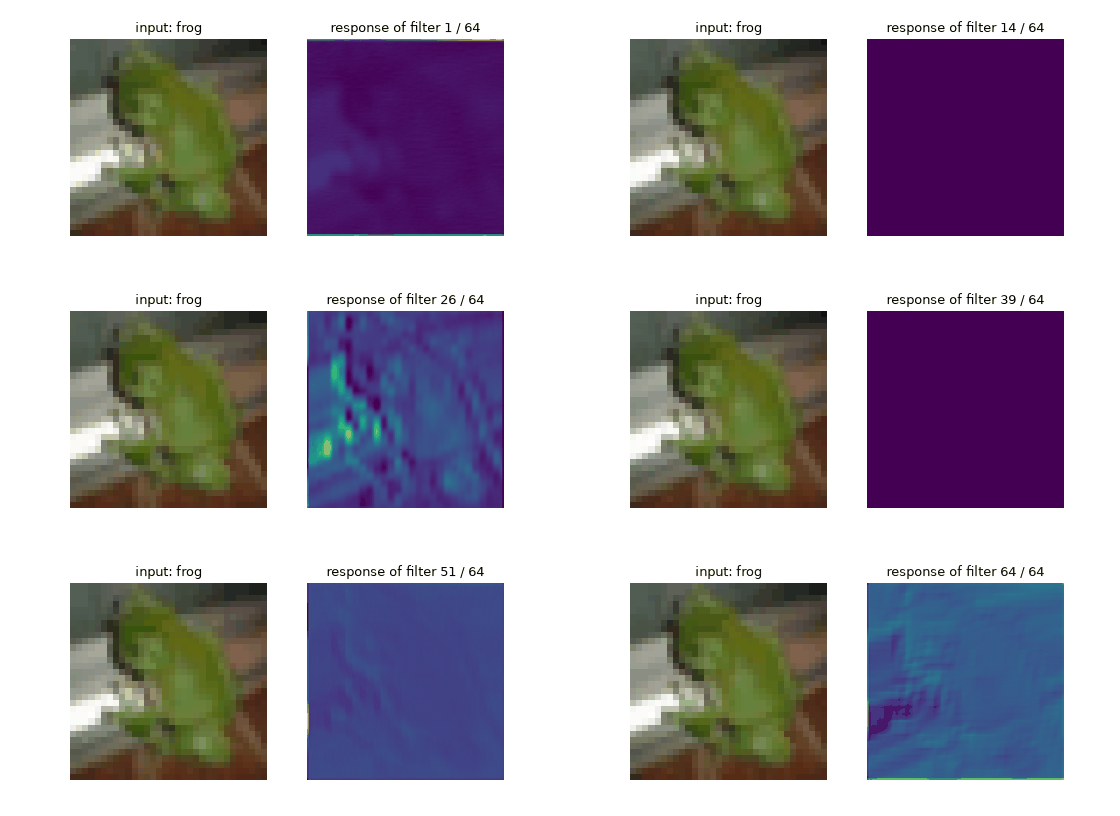Each of the 64 first-layer ImageNet filters responding to the same input image.

3. Dataset Preparation¶

We will classify three CIFAR-10 classes — cat, dog and ship — using only a few hundred labelled images per class, which is exactly the situation transfer learning is designed for.

Two details matter more than they look:

1. Match the preprocessing to the weights. A pretrained network expects the same input statistics it was trained on: 224x224 pixels, RGB, normalised with the ImageNet mean and standard deviation. weights.transforms() gives you exactly that pipeline. Feeding it raw 32x32 CIFAR images would waste most of what it knows.
2. Augment the training set, not the test set. Random flips and crops multiply your limited data; applying them at test time would just add noise to the evaluation.

In [6]:

CLASSES = ['cat', 'dog', 'ship']
N_PER_CLASS_TRAIN = 300      # deliberately small - this is the point of the lab
N_PER_CLASS_TEST = 150
IMG_SIZE = 160               # smaller than ImageNet's 224 to keep CPU training bearable

IMAGENET_MEAN = [0.485, 0.456, 0.406]
IMAGENET_STD = [0.229, 0.224, 0.225]

train_tf = transforms.Compose([
    transforms.Resize((IMG_SIZE, IMG_SIZE)),
    transforms.RandomHorizontalFlip(),
    transforms.RandomAffine(degrees=8, translate=(0.06, 0.06)),
    transforms.ToTensor(),
    transforms.Normalize(IMAGENET_MEAN, IMAGENET_STD),
])

test_tf = transforms.Compose([
    transforms.Resize((IMG_SIZE, IMG_SIZE)),
    transforms.ToTensor(),
    transforms.Normalize(IMAGENET_MEAN, IMAGENET_STD),
])

CLASSES = ['cat', 'dog', 'ship'] N_PER_CLASS_TRAIN = 300 # deliberately small - this is the point of the lab N_PER_CLASS_TEST = 150 IMG_SIZE = 160 # smaller than ImageNet's 224 to keep CPU training bearable IMAGENET_MEAN = [0.485, 0.456, 0.406] IMAGENET_STD = [0.229, 0.224, 0.225] train_tf = transforms.Compose([ transforms.Resize((IMG_SIZE, IMG_SIZE)), transforms.RandomHorizontalFlip(), transforms.RandomAffine(degrees=8, translate=(0.06, 0.06)), transforms.ToTensor(), transforms.Normalize(IMAGENET_MEAN, IMAGENET_STD), ]) test_tf = transforms.Compose([ transforms.Resize((IMG_SIZE, IMG_SIZE)), transforms.ToTensor(), transforms.Normalize(IMAGENET_MEAN, IMAGENET_STD), ])

In [7]:

def few_shot_subset(train, n_per_class, tf, seed=0):
    """Take the first n_per_class images of each wanted class and relabel them 0..k-1."""
    base = datasets.CIFAR10(root='./data', train=train, download=True, transform=tf)
    wanted = {base.class_to_idx[c]: i for i, c in enumerate(CLASSES)}

    rng = np.random.default_rng(seed)
    targets = np.array(base.targets)
    indices = []
    for orig_label in wanted:
        pool = np.where(targets == orig_label)[0]
        indices.extend(rng.choice(pool, size=n_per_class, replace=False).tolist())
    rng.shuffle(indices)

    # remap CIFAR's label ids onto 0, 1, 2
    base.targets = [wanted.get(t, -1) for t in base.targets]
    return Subset(base, indices)

train_set = few_shot_subset(True, N_PER_CLASS_TRAIN, train_tf, seed=0)
test_set = few_shot_subset(False, N_PER_CLASS_TEST, test_tf, seed=1)

train_loader = DataLoader(train_set, batch_size=32, shuffle=True, num_workers=0)
test_loader = DataLoader(test_set, batch_size=64, shuffle=False, num_workers=0)

print(f'{len(train_set)} training images, {len(test_set)} test images, {len(CLASSES)} classes')
print('That is roughly 0.5% of the data a from-scratch CNN would want.')

def few_shot_subset(train, n_per_class, tf, seed=0): """Take the first n_per_class images of each wanted class and relabel them 0..k-1.""" base = datasets.CIFAR10(root='./data', train=train, download=True, transform=tf) wanted = {base.class_to_idx[c]: i for i, c in enumerate(CLASSES)} rng = np.random.default_rng(seed) targets = np.array(base.targets) indices = [] for orig_label in wanted: pool = np.where(targets == orig_label)[0] indices.extend(rng.choice(pool, size=n_per_class, replace=False).tolist()) rng.shuffle(indices) # remap CIFAR's label ids onto 0, 1, 2 base.targets = [wanted.get(t, -1) for t in base.targets] return Subset(base, indices) train_set = few_shot_subset(True, N_PER_CLASS_TRAIN, train_tf, seed=0) test_set = few_shot_subset(False, N_PER_CLASS_TEST, test_tf, seed=1) train_loader = DataLoader(train_set, batch_size=32, shuffle=True, num_workers=0) test_loader = DataLoader(test_set, batch_size=64, shuffle=False, num_workers=0) print(f'{len(train_set)} training images, {len(test_set)} test images, {len(CLASSES)} classes') print('That is roughly 0.5% of the data a from-scratch CNN would want.')

C:\Users\injye\.conda\envs\envNeural\Lib\site-packages\torchvision\datasets\cifar.py:83: VisibleDeprecationWarning: dtype(): align should be passed as Python or NumPy boolean but got `align=0`. Did you mean to pass a tuple to create a subarray type? (Deprecated NumPy 2.4)
  entry = pickle.load(f, encoding="latin1")

900 training images, 450 test images, 3 classes
That is roughly 0.5% of the data a from-scratch CNN would want.

In [8]:

# Look at a batch (undoing the normalisation so the colours are right)
def denormalize(t):
    mean = torch.tensor(IMAGENET_MEAN).view(3, 1, 1)
    std = torch.tensor(IMAGENET_STD).view(3, 1, 1)
    return (t * std + mean).clamp(0, 1)

images, labels = next(iter(train_loader))
fig, axes = plt.subplots(1, 8, figsize=(12, 2))
for ax, img, lab in zip(axes, images, labels):
    ax.imshow(denormalize(img).permute(1, 2, 0).numpy())
    ax.set_title(CLASSES[lab], fontsize=9)
    ax.axis('off')
plt.tight_layout()
plt.show()

# Look at a batch (undoing the normalisation so the colours are right) def denormalize(t): mean = torch.tensor(IMAGENET_MEAN).view(3, 1, 1) std = torch.tensor(IMAGENET_STD).view(3, 1, 1) return (t * std + mean).clamp(0, 1) images, labels = next(iter(train_loader)) fig, axes = plt.subplots(1, 8, figsize=(12, 2)) for ax, img, lab in zip(axes, images, labels): ax.imshow(denormalize(img).permute(1, 2, 0).numpy()) ax.set_title(CLASSES[lab], fontsize=9) ax.axis('off') plt.tight_layout() plt.show()

4. Approach A: Feature Extraction¶

Freeze everything, throw away the 1,000-class ImageNet head, and bolt on a fresh nn.Linear for our three classes.

Setting requires_grad = False tells autograd not to compute gradients for those tensors. They will not be updated, and the backward pass gets cheaper. Note that a newly created layer always has requires_grad = True, so replacing fc after freezing gives us exactly the split we want.

In [9]:

def build_feature_extractor(num_classes=len(CLASSES)):
    model = models.resnet18(weights=models.ResNet18_Weights.DEFAULT)
    for param in model.parameters():
        param.requires_grad = False          # freeze the whole backbone
    in_features = model.fc.in_features       # 512 for ResNet-18
    model.fc = nn.Linear(in_features, num_classes)   # brand new, trainable
    return model

fe_model = build_feature_extractor().to(device)

trainable = sum(p.numel() for p in fe_model.parameters() if p.requires_grad)
frozen = sum(p.numel() for p in fe_model.parameters() if not p.requires_grad)
print(f'Trainable parameters: {trainable:,}')
print(f'Frozen parameters   : {frozen:,}')
print(f'We are training {100 * trainable / (trainable + frozen):.2f}% of the network.')

def build_feature_extractor(num_classes=len(CLASSES)): model = models.resnet18(weights=models.ResNet18_Weights.DEFAULT) for param in model.parameters(): param.requires_grad = False # freeze the whole backbone in_features = model.fc.in_features # 512 for ResNet-18 model.fc = nn.Linear(in_features, num_classes) # brand new, trainable return model fe_model = build_feature_extractor().to(device) trainable = sum(p.numel() for p in fe_model.parameters() if p.requires_grad) frozen = sum(p.numel() for p in fe_model.parameters() if not p.requires_grad) print(f'Trainable parameters: {trainable:,}') print(f'Frozen parameters : {frozen:,}') print(f'We are training {100 * trainable / (trainable + frozen):.2f}% of the network.')

Trainable parameters: 1,539
Frozen parameters   : 11,176,512
We are training 0.01% of the network.

A reusable training loop¶

Every lab from here on needs the same loop, so let's write it once. Two details specific to transfer learning:

• We pass only the trainable parameters to the optimizer. Handing it frozen ones is harmless but misleading.
• We keep the frozen BatchNorm layers in eval() mode during fine-tuning later, so their running statistics are not overwritten by our tiny batches.

In [10]:

criterion = nn.CrossEntropyLoss()

def evaluate(model, loader):
    model.eval()
    correct = total = 0
    with torch.no_grad():
        for images, labels in loader:
            images, labels = images.to(device), labels.to(device)
            preds = model(images).argmax(dim=1)
            correct += (preds == labels).sum().item()
            total += labels.size(0)
    return 100 * correct / total

def train_model(model, epochs=4, lr=1e-3, params=None, label=''):
    params = params if params is not None else [p for p in model.parameters() if p.requires_grad]
    optimizer = optim.Adam(params, lr=lr)
    history = []
    for epoch in range(epochs):
        model.train()
        running = 0.0
        for images, labels in train_loader:
            images, labels = images.to(device), labels.to(device)
            optimizer.zero_grad()
            loss = criterion(model(images), labels)
            loss.backward()
            optimizer.step()
            running += loss.item() * images.size(0)
        acc = evaluate(model, test_loader)
        history.append(acc)
        print(f'  [{label}] epoch {epoch+1}/{epochs}  '
              f'loss {running/len(train_set):.4f}  test acc {acc:.2f}%')
    return history

criterion = nn.CrossEntropyLoss() def evaluate(model, loader): model.eval() correct = total = 0 with torch.no_grad(): for images, labels in loader: images, labels = images.to(device), labels.to(device) preds = model(images).argmax(dim=1) correct += (preds == labels).sum().item() total += labels.size(0) return 100 * correct / total def train_model(model, epochs=4, lr=1e-3, params=None, label=''): params = params if params is not None else [p for p in model.parameters() if p.requires_grad] optimizer = optim.Adam(params, lr=lr) history = [] for epoch in range(epochs): model.train() running = 0.0 for images, labels in train_loader: images, labels = images.to(device), labels.to(device) optimizer.zero_grad() loss = criterion(model(images), labels) loss.backward() optimizer.step() running += loss.item() * images.size(0) acc = evaluate(model, test_loader) history.append(acc) print(f' [{label}] epoch {epoch+1}/{epochs} ' f'loss {running/len(train_set):.4f} test acc {acc:.2f}%') return history

In [11]:

import time

print('Feature extraction (backbone frozen):')
t0 = time.time()
fe_history = train_model(fe_model, epochs=4, lr=1e-3, label='frozen')
fe_time = time.time() - t0
print(f'Finished in {fe_time:.1f}s, final accuracy {fe_history[-1]:.2f}%')

import time print('Feature extraction (backbone frozen):') t0 = time.time() fe_history = train_model(fe_model, epochs=4, lr=1e-3, label='frozen') fe_time = time.time() - t0 print(f'Finished in {fe_time:.1f}s, final accuracy {fe_history[-1]:.2f}%')

Feature extraction (backbone frozen):

  [frozen] epoch 1/4  loss 0.8484  test acc 72.89%

  [frozen] epoch 2/4  loss 0.5365  test acc 78.44%

  [frozen] epoch 3/4  loss 0.4644  test acc 84.67%

  [frozen] epoch 4/4  loss 0.4039  test acc 84.67%
Finished in 109.1s, final accuracy 84.67%

5. Approach B: Fine-Tuning¶

Feature extraction treats the backbone as a fixed function. Fine-tuning lets the last part of it adapt to our data.

Three rules keep it from going wrong:

1. Train the head first (which we just did). An untrained head produces large, meaningless gradients that would wreck good pretrained weights on the very first batch.
2. Use a much smaller learning rate for the backbone — typically 10x smaller. We want to nudge those weights, not retrain them.
3. Unfreeze from the top down. The last block is the most task-specific and the safest to change; the first layers detect edges and are already right.

PyTorch supports different learning rates per group directly, by passing a list of dicts to the optimizer.

In [12]:

# Continue from the feature-extraction model, now unfreezing the last residual block
ft_model = fe_model

for param in ft_model.layer4.parameters():
    param.requires_grad = True

param_groups = [
    {'params': ft_model.layer4.parameters(), 'lr': 1e-4},   # gentle on pretrained weights
    {'params': ft_model.fc.parameters(), 'lr': 1e-3},       # the head can still move fast
]

trainable = sum(p.numel() for p in ft_model.parameters() if p.requires_grad)
print(f'Now training {trainable:,} parameters (layer4 + fc)')

# Continue from the feature-extraction model, now unfreezing the last residual block ft_model = fe_model for param in ft_model.layer4.parameters(): param.requires_grad = True param_groups = [ {'params': ft_model.layer4.parameters(), 'lr': 1e-4}, # gentle on pretrained weights {'params': ft_model.fc.parameters(), 'lr': 1e-3}, # the head can still move fast ] trainable = sum(p.numel() for p in ft_model.parameters() if p.requires_grad) print(f'Now training {trainable:,} parameters (layer4 + fc)')

Now training 8,395,267 parameters (layer4 + fc)

In [13]:

def train_with_groups(model, groups, epochs=4, label=''):
    optimizer = optim.Adam(groups)
    history = []
    for epoch in range(epochs):
        model.train()
        # keep frozen BatchNorm layers from updating their running statistics
        for module in model.modules():
            if isinstance(module, nn.BatchNorm2d) and not module.weight.requires_grad:
                module.eval()
        running = 0.0
        for images, labels in train_loader:
            images, labels = images.to(device), labels.to(device)
            optimizer.zero_grad()
            loss = criterion(model(images), labels)
            loss.backward()
            optimizer.step()
            running += loss.item() * images.size(0)
        acc = evaluate(model, test_loader)
        history.append(acc)
        print(f'  [{label}] epoch {epoch+1}/{epochs}  '
              f'loss {running/len(train_set):.4f}  test acc {acc:.2f}%')
    return history

print('Fine-tuning (layer4 unfrozen):')
t0 = time.time()
ft_history = train_with_groups(ft_model, param_groups, epochs=4, label='fine-tune')
ft_time = time.time() - t0
print(f'Finished in {ft_time:.1f}s, final accuracy {ft_history[-1]:.2f}%')

def train_with_groups(model, groups, epochs=4, label=''): optimizer = optim.Adam(groups) history = [] for epoch in range(epochs): model.train() # keep frozen BatchNorm layers from updating their running statistics for module in model.modules(): if isinstance(module, nn.BatchNorm2d) and not module.weight.requires_grad: module.eval() running = 0.0 for images, labels in train_loader: images, labels = images.to(device), labels.to(device) optimizer.zero_grad() loss = criterion(model(images), labels) loss.backward() optimizer.step() running += loss.item() * images.size(0) acc = evaluate(model, test_loader) history.append(acc) print(f' [{label}] epoch {epoch+1}/{epochs} ' f'loss {running/len(train_set):.4f} test acc {acc:.2f}%') return history print('Fine-tuning (layer4 unfrozen):') t0 = time.time() ft_history = train_with_groups(ft_model, param_groups, epochs=4, label='fine-tune') ft_time = time.time() - t0 print(f'Finished in {ft_time:.1f}s, final accuracy {ft_history[-1]:.2f}%')

Fine-tuning (layer4 unfrozen):

  [fine-tune] epoch 1/4  loss 0.3700  test acc 85.78%

  [fine-tune] epoch 2/4  loss 0.2210  test acc 86.44%

  [fine-tune] epoch 3/4  loss 0.1693  test acc 87.11%

  [fine-tune] epoch 4/4  loss 0.1291  test acc 85.78%
Finished in 119.3s, final accuracy 85.78%

6. The Baseline: Training From Scratch¶

None of the above means anything without a control. The same ResNet-18 architecture, the same data, the same number of epochs — but starting from random weights.

In [14]:

scratch_model = models.resnet18(weights=None)               # random initialisation
scratch_model.fc = nn.Linear(scratch_model.fc.in_features, len(CLASSES))
scratch_model = scratch_model.to(device)

print('From scratch (random initialisation):')
t0 = time.time()
scratch_history = train_model(scratch_model, epochs=4, lr=1e-3, label='scratch')
scratch_time = time.time() - t0
print(f'Finished in {scratch_time:.1f}s, final accuracy {scratch_history[-1]:.2f}%')

scratch_model = models.resnet18(weights=None) # random initialisation scratch_model.fc = nn.Linear(scratch_model.fc.in_features, len(CLASSES)) scratch_model = scratch_model.to(device) print('From scratch (random initialisation):') t0 = time.time() scratch_history = train_model(scratch_model, epochs=4, lr=1e-3, label='scratch') scratch_time = time.time() - t0 print(f'Finished in {scratch_time:.1f}s, final accuracy {scratch_history[-1]:.2f}%')

From scratch (random initialisation):

  [scratch] epoch 1/4  loss 1.0647  test acc 54.89%

  [scratch] epoch 2/4  loss 0.7777  test acc 52.22%

  [scratch] epoch 3/4  loss 0.7392  test acc 65.33%

  [scratch] epoch 4/4  loss 0.6999  test acc 60.44%
Finished in 204.4s, final accuracy 60.44%

In [15]:

fig, (ax1, ax2) = plt.subplots(1, 2, figsize=(11, 4))

epochs = range(1, len(fe_history) + 1)
ax1.plot(epochs, scratch_history, marker='s', label='from scratch')
ax1.plot(epochs, fe_history, marker='o', label='feature extraction')
ax1.plot(range(len(fe_history) + 1, len(fe_history) + len(ft_history) + 1),
         ft_history, marker='^', label='fine-tuning (continues)')
ax1.axhline(100 / len(CLASSES), color='gray', linestyle=':', label='chance')
ax1.set_xlabel('Epoch')
ax1.set_ylabel('Test accuracy (%)')
ax1.set_title('Same data, same architecture')
ax1.legend(fontsize=9)
ax1.grid(alpha=0.3)

names = ['scratch', 'frozen', 'fine-tuned']
finals = [scratch_history[-1], fe_history[-1], ft_history[-1]]
ax2.bar(names, finals, color=['#C44E52', '#4C72B0', '#55A868'])
for i, v in enumerate(finals):
    ax2.text(i, v + 1, f'{v:.1f}%', ha='center')
ax2.axhline(100 / len(CLASSES), color='gray', linestyle=':')
ax2.set_ylim(0, 105)
ax2.set_ylabel('Final test accuracy (%)')
ax2.set_title(f'{N_PER_CLASS_TRAIN} images per class')
plt.tight_layout()
plt.show()

fig, (ax1, ax2) = plt.subplots(1, 2, figsize=(11, 4)) epochs = range(1, len(fe_history) + 1) ax1.plot(epochs, scratch_history, marker='s', label='from scratch') ax1.plot(epochs, fe_history, marker='o', label='feature extraction') ax1.plot(range(len(fe_history) + 1, len(fe_history) + len(ft_history) + 1), ft_history, marker='^', label='fine-tuning (continues)') ax1.axhline(100 / len(CLASSES), color='gray', linestyle=':', label='chance') ax1.set_xlabel('Epoch') ax1.set_ylabel('Test accuracy (%)') ax1.set_title('Same data, same architecture') ax1.legend(fontsize=9) ax1.grid(alpha=0.3) names = ['scratch', 'frozen', 'fine-tuned'] finals = [scratch_history[-1], fe_history[-1], ft_history[-1]] ax2.bar(names, finals, color=['#C44E52', '#4C72B0', '#55A868']) for i, v in enumerate(finals): ax2.text(i, v + 1, f'{v:.1f}%', ha='center') ax2.axhline(100 / len(CLASSES), color='gray', linestyle=':') ax2.set_ylim(0, 105) ax2.set_ylabel('Final test accuracy (%)') ax2.set_title(f'{N_PER_CLASS_TRAIN} images per class') plt.tight_layout() plt.show()

With only a few hundred images per class, the from-scratch network has nowhere near enough data and lands close to chance. The pretrained backbone gets most of the way there in a single epoch, because it never had to learn what an edge is.

7. Where the Model Goes Wrong¶

Accuracy is one number and it hides everything interesting. A confusion matrix shows which classes get mixed up — and here the answer is predictable: cats and dogs look alike, ships do not look like either.

In [16]:

ft_model.eval()
n = len(CLASSES)
confusion = np.zeros((n, n), dtype=int)
wrong = []

with torch.no_grad():
    for images, labels in test_loader:
        preds = ft_model(images.to(device)).argmax(dim=1).cpu()
        for img, true, pred in zip(images, labels, preds):
            confusion[true, pred] += 1
            if true != pred and len(wrong) < 8:
                wrong.append((img, true.item(), pred.item()))

fig, ax = plt.subplots(figsize=(4.5, 4))
ax.imshow(confusion, cmap='Blues')
ax.set_xticks(range(n), CLASSES)
ax.set_yticks(range(n), CLASSES)
ax.set_xlabel('predicted')
ax.set_ylabel('actual')
ax.set_title('Confusion matrix')
for i in range(n):
    for j in range(n):
        ax.text(j, i, confusion[i, j], ha='center', va='center',
                color='white' if confusion[i, j] > confusion.max() / 2 else 'black')
plt.tight_layout()
plt.show()

ft_model.eval() n = len(CLASSES) confusion = np.zeros((n, n), dtype=int) wrong = [] with torch.no_grad(): for images, labels in test_loader: preds = ft_model(images.to(device)).argmax(dim=1).cpu() for img, true, pred in zip(images, labels, preds): confusion[true, pred] += 1 if true != pred and len(wrong) < 8: wrong.append((img, true.item(), pred.item())) fig, ax = plt.subplots(figsize=(4.5, 4)) ax.imshow(confusion, cmap='Blues') ax.set_xticks(range(n), CLASSES) ax.set_yticks(range(n), CLASSES) ax.set_xlabel('predicted') ax.set_ylabel('actual') ax.set_title('Confusion matrix') for i in range(n): for j in range(n): ax.text(j, i, confusion[i, j], ha='center', va='center', color='white' if confusion[i, j] > confusion.max() / 2 else 'black') plt.tight_layout() plt.show()

In [17]:

if wrong:
    fig, axes = plt.subplots(1, len(wrong), figsize=(1.6 * len(wrong), 2.2))
    axes = np.atleast_1d(axes)
    for ax, (img, true, pred) in zip(axes, wrong):
        ax.imshow(denormalize(img).permute(1, 2, 0).numpy())
        ax.set_title(f'{CLASSES[true]}\n-> {CLASSES[pred]}', fontsize=8)
        ax.axis('off')
    fig.suptitle('Misclassified test images')
    plt.tight_layout()
    plt.show()
else:
    print('No misclassified images in the test set.')

if wrong: fig, axes = plt.subplots(1, len(wrong), figsize=(1.6 * len(wrong), 2.2)) axes = np.atleast_1d(axes) for ax, (img, true, pred) in zip(axes, wrong): ax.imshow(denormalize(img).permute(1, 2, 0).numpy()) ax.set_title(f'{CLASSES[true]}\n-> {CLASSES[pred]}', fontsize=8) ax.axis('off') fig.suptitle('Misclassified test images') plt.tight_layout() plt.show() else: print('No misclassified images in the test set.')

8. Saving and Loading the Model¶

Save the state_dict, not the model object. Pickling the whole model ties the file to your exact class definitions and file layout, and it breaks the moment you refactor. A state_dict is just a dictionary of tensors, and it survives.

To load it you rebuild the architecture first, then pour the weights in.

In [18]:

torch.save({
    'state_dict': ft_model.state_dict(),
    'classes': CLASSES,
    'img_size': IMG_SIZE,
}, 'transfer_resnet18.pt')

# Loading it back: rebuild the same architecture, then load the tensors
checkpoint = torch.load('transfer_resnet18.pt', map_location=device, weights_only=True)

loaded = models.resnet18(weights=None)
loaded.fc = nn.Linear(loaded.fc.in_features, len(checkpoint['classes']))
loaded.load_state_dict(checkpoint['state_dict'])
loaded = loaded.to(device)

print('Reloaded model accuracy:', f'{evaluate(loaded, test_loader):.2f}%')
print('Saved classes:', checkpoint['classes'])

torch.save({ 'state_dict': ft_model.state_dict(), 'classes': CLASSES, 'img_size': IMG_SIZE, }, 'transfer_resnet18.pt') # Loading it back: rebuild the same architecture, then load the tensors checkpoint = torch.load('transfer_resnet18.pt', map_location=device, weights_only=True) loaded = models.resnet18(weights=None) loaded.fc = nn.Linear(loaded.fc.in_features, len(checkpoint['classes'])) loaded.load_state_dict(checkpoint['state_dict']) loaded = loaded.to(device) print('Reloaded model accuracy:', f'{evaluate(loaded, test_loader):.2f}%') print('Saved classes:', checkpoint['classes'])

Reloaded model accuracy: 85.78%
Saved classes: ['cat', 'dog', 'ship']

9. Experiment: Try Different Architectures and Hyperparameters¶

You can experiment with:

• Dropping N_PER_CLASS_TRAIN to 50 or 25 — how far can transfer learning be pushed before it breaks?
• Unfreezing layer3 as well, with an even smaller learning rate
• Swapping ResNet-18 for models.efficientnet_b0 or models.mobilenet_v3_small (the head attribute is named classifier, not fc — check with print(model))
• Replacing the single nn.Linear head with nn.Sequential(nn.Dropout(0.3), nn.Linear(512, 3))
• Precomputing the frozen features once and training only the linear head on them: with a frozen backbone the features never change, so this turns four epochs of convolution into a few seconds of matrix algebra
• Removing the augmentation transforms and watching the overfitting appear
• Adding harder classes (CLASSES = ['cat', 'dog', 'deer', 'horse']) and seeing where the confusion matrix fills in

Try modifying the model definition or training loop above and observe how the performance changes.

10. Conclusion¶

In this lab, you learned how to reuse a pretrained network instead of starting from random weights. You froze a ResNet-18 backbone and trained a new head on a few hundred images, then fine-tuned the last block at a reduced learning rate, and compared both against training the same architecture from scratch.

Key takeaways:

• Early CNN layers learn general visual features; only the last layers are task-specific.
• requires_grad = False freezes a tensor; create the new head after freezing so it stays trainable.
• Preprocess your images the way the pretrained weights expect, or you throw away most of the benefit.
• Train the head before unfreezing anything, and fine-tune with a much lower learning rate.
• Save the state_dict, not the model object.

Transfer learning is the default starting point for almost every real computer vision project. The next lab steps back from architectures and looks at the techniques that decide whether any network you train will generalise: regularization and optimization.