Lab 09: Convolutional Neural Networks (CNN)¶

In this lab, you will learn about Convolutional Neural Networks (CNNs), a powerful class of deep learning models widely used for image classification and computer vision tasks. You will understand the basic building blocks of CNNs, implement a simple CNN using PyTorch, and train it on an image dataset.

We will cover the following topics:

• Understanding the structure and intuition behind CNNs
• Implementing a basic CNN with PyTorch
• Training and evaluating the CNN on a dataset
• Experimenting with different architectures and hyperparameters

1. What is a Convolutional Neural Network (CNN)?¶

A Convolutional Neural Network (CNN) is a type of deep learning model designed to process data with a grid-like topology, such as images. CNNs are especially effective for image classification, object detection, and other computer vision tasks.

Key components of a CNN:

• Convolutional layers: Apply filters to extract features from the input image.
• Activation functions: Introduce non-linearity (e.g., ReLU).
• Pooling layers: Downsample feature maps to reduce dimensionality and computation.
• Fully connected layers: Combine features for final classification or regression.

CNNs learn to automatically extract hierarchical features from raw input data, making them highly effective for visual recognition tasks.

A typical Convolutional Neural Network (CNN) architecture. The network consists of convolutional layers, pooling layers, and fully connected layers. Diagram redrawn locally; the original was hot-linked and is no longer served.

2. Intuition and Workflow of CNNs¶

CNNs work by learning spatial hierarchies of features from input images. Early layers detect simple patterns (edges, colors), while deeper layers capture complex structures (shapes, objects).

Typical workflow:

1. Input image: The raw image is fed into the network.
2. Convolution: Filters scan the image to produce feature maps.
3. Activation: Non-linear functions (e.g., ReLU) are applied to introduce non-linearity.
4. Pooling: Feature maps are downsampled to reduce size and computation.
5. Flattening: The output is flattened into a vector.
6. Fully connected layers: The vector is processed for final classification or regression.

How Convolution Works in CNNs¶

The convolution operation is the core building block of a CNN. It allows the network to extract local features from the input image by sliding a small filter (kernel) over the image and computing dot products.

Step-by-step workflow:

1. Filter (Kernel): A small matrix of weights (e.g., 3x3 or 5x5) that is learned during training.
2. Sliding Window: The filter moves (slides) across the input image, one small region at a time (this region is called the receptive field).
3. Element-wise Multiplication: At each position, the filter and the corresponding region of the image are multiplied element-wise and summed up to produce a single value.
4. Feature Map: The result of the convolution at each position forms a new matrix called a feature map (or activation map).
5. Multiple Filters: Multiple filters are used to extract different types of features (e.g., edges, textures, shapes). Each filter produces its own feature map.
6. Stride and Padding: The stride determines how far the filter moves at each step. Padding can be added to the input image to control the spatial size of the output feature map.

This process enables CNNs to detect patterns regardless of their position in the image, making them highly effective for visual tasks.

Visualization: A filter (kernel) slides over the input image, performing element-wise multiplication and summing the results to create a feature map.

What is Pooling in CNNs?¶

Pooling is a downsampling operation used in CNNs to reduce the spatial dimensions (width and height) of feature maps. This helps decrease the number of parameters, control overfitting, and make the network more robust to small translations in the input.

Types of pooling:

• Max Pooling: Takes the maximum value from each patch of the feature map.
• Average Pooling: Takes the average value from each patch.

How it works: A pooling layer slides a window (e.g., 2x2) over the input feature map and replaces the region with a single value (max or average).

In this example, each 2x2 region is replaced by its maximum value. Pooling reduces the feature map size, making the network more efficient and less sensitive to small shifts in the input.

In [1]:

# Example: Max Pooling with PyTorch
import torch
import torch.nn as nn

# Example input: 1 sample, 1 channel, 4x4 feature map
x = torch.tensor([[[[1.0, 2.0, 3.0, 4.0],
                    [5.0, 6.0, 7.0, 8.0],
                    [9.0, 10.0, 11.0, 12.0],
                    [13.0, 14.0, 15.0, 16.0]]]])

# Max pooling layer with 2x2 window and stride 2
pool = nn.MaxPool2d(kernel_size=2, stride=2)
output = pool(x)
print(output)

# Example: Max Pooling with PyTorch import torch import torch.nn as nn # Example input: 1 sample, 1 channel, 4x4 feature map x = torch.tensor([[[[1.0, 2.0, 3.0, 4.0], [5.0, 6.0, 7.0, 8.0], [9.0, 10.0, 11.0, 12.0], [13.0, 14.0, 15.0, 16.0]]]]) # Max pooling layer with 2x2 window and stride 2 pool = nn.MaxPool2d(kernel_size=2, stride=2) output = pool(x) print(output)

tensor([[[[ 6.,  8.],
          [14., 16.]]]])

Visualization: Diagram redrawn locally; the original was hot-linked and is no longer served.

What is Flattening in CNNs?¶

Flattening is the process of converting a multi-dimensional tensor (such as a 3D feature map) into a 1D vector. This step is necessary before passing the data from convolutional and pooling layers to fully connected (dense) layers, which expect 1D input. 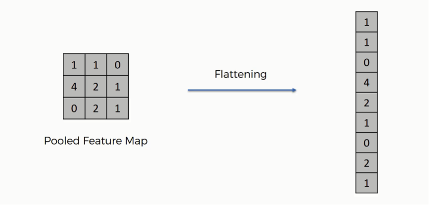Source: superdatascience.com Why flatten?

• Convolutional and pooling layers output 3D tensors (channels, height, width).
• Fully connected layers require 1D vectors as input.
• Flattening bridges this gap by reshaping the tensor.

Example: Flattening with PyTorch

In this example, each 3x4x4 feature map is flattened into a 1D vector of length 48 (344), ready to be fed into a fully connected layer.

In [2]:

# Example: Flattening a tensor in PyTorch
import torch

# Example input: batch of 2 samples, 3 channels, 4x4 feature maps
x = torch.randn(2, 3, 4, 4)
print('Original shape:', x.shape)

# Flatten each sample to a 1D vector
x_flat = x.view(x.size(0), -1)
print('Flattened shape:', x_flat.shape)

# Example: Flattening a tensor in PyTorch import torch # Example input: batch of 2 samples, 3 channels, 4x4 feature maps x = torch.randn(2, 3, 4, 4) print('Original shape:', x.shape) # Flatten each sample to a 1D vector x_flat = x.view(x.size(0), -1) print('Flattened shape:', x_flat.shape)

Original shape: torch.Size([2, 3, 4, 4])
Flattened shape: torch.Size([2, 48])

When building CNNs in PyTorch, the forward method defines how data flows through the network. After several convolutional and pooling layers, the output is typically a multi-dimensional tensor (batch size, channels, height, width). To connect this output to fully connected (dense) layers, you must flatten each sample into a 1D vector. This is done using the view method:

In [3]:

x = x.view(x.size(0), -1)  # Flatten all dimensions except batch

x = x.view(x.size(0), -1) # Flatten all dimensions except batch

• x.size(0) is the batch size, so each sample in the batch is flattened independently.
• -1 tells PyTorch to infer the correct length for the flattened vector.

Why is this necessary?

• Fully connected layers expect input of shape (batch_size, num_features).
• Flattening ensures the output from the convolutional part matches this shape.

Without flattening, you would get a shape mismatch error when passing the output of the convolutional layers to the fully connected layer. Flattening is a crucial step that bridges the convolutional and dense parts of a neural network.

Example in a PyTorch model:

In [4]:

import torch.nn.functional as F

class SimpleCNN(nn.Module):
    def __init__(self):
        super(SimpleCNN, self).__init__()
        self.conv1 = nn.Conv2d(1, 16, kernel_size=3, padding=1)
        self.pool = nn.MaxPool2d(2, 2)
        self.fc1 = nn.Linear(16 * 14 * 14, 10)  # for 28x28 input images
    
    def forward(self, x):
        x = self.pool(F.relu(self.conv1(x)))
        x = x.view(x.size(0), -1)  # Flatten before the fully connected layer
        x = self.fc1(x)
        return x

import torch.nn.functional as F class SimpleCNN(nn.Module): def __init__(self): super(SimpleCNN, self).__init__() self.conv1 = nn.Conv2d(1, 16, kernel_size=3, padding=1) self.pool = nn.MaxPool2d(2, 2) self.fc1 = nn.Linear(16 * 14 * 14, 10) # for 28x28 input images def forward(self, x): x = self.pool(F.relu(self.conv1(x))) x = x.view(x.size(0), -1) # Flatten before the fully connected layer x = self.fc1(x) return x

3. Introduction to PyTorch for CNNs¶

PyTorch is a popular deep learning library that makes it easy to build and train CNNs. In this lab, you will use PyTorch to:

• Define a simple CNN model
• Train the model on an image dataset
• Evaluate its performance

In [5]:

# Import PyTorch and check version
import torch
import torch.nn as nn
import torch.optim as optim
print('PyTorch version:', torch.__version__)

# Import PyTorch and check version import torch import torch.nn as nn import torch.optim as optim print('PyTorch version:', torch.__version__)

PyTorch version: 2.13.0+cpu

4. Dataset Preparation¶

For this lab, we will use the MNIST dataset, a classic benchmark for handwritten digit recognition. PyTorch provides utilities to easily download and load this dataset.

In [6]:

# Download and load the MNIST dataset
from torchvision import datasets, transforms
from torch.utils.data import DataLoader

# Define transformations for the data
transform = transforms.Compose([
    transforms.ToTensor(),
    transforms.Normalize((0.1307,), (0.3081,)) # mean and std for MNIST
])

# Download training and test datasets
train_dataset = datasets.MNIST(root='./data', train=True, download=True, transform=transform)
test_dataset = datasets.MNIST(root='./data', train=False, download=True, transform=transform)

# Create data loaders
train_loader = DataLoader(train_dataset, batch_size=64, shuffle=True)
test_loader = DataLoader(test_dataset, batch_size=1000, shuffle=False)

# Download and load the MNIST dataset from torchvision import datasets, transforms from torch.utils.data import DataLoader # Define transformations for the data transform = transforms.Compose([ transforms.ToTensor(), transforms.Normalize((0.1307,), (0.3081,)) # mean and std for MNIST ]) # Download training and test datasets train_dataset = datasets.MNIST(root='./data', train=True, download=True, transform=transform) test_dataset = datasets.MNIST(root='./data', train=False, download=True, transform=transform) # Create data loaders train_loader = DataLoader(train_dataset, batch_size=64, shuffle=True) test_loader = DataLoader(test_dataset, batch_size=1000, shuffle=False)

In [7]:

# Visualize some MNIST images
import matplotlib.pyplot as plt
import numpy as np

examples = enumerate(train_loader)
batch_idx, (example_data, example_targets) = next(examples)

fig = plt.figure(figsize=(8, 2))
for i in range(8):
    plt.subplot(1, 8, i+1)
    plt.tight_layout()
    plt.imshow(example_data[i][0], cmap='gray', interpolation='none')
    plt.title(f"{example_targets[i].item()}")
    plt.xticks([])
    plt.yticks([])
plt.show()

# Visualize some MNIST images import matplotlib.pyplot as plt import numpy as np examples = enumerate(train_loader) batch_idx, (example_data, example_targets) = next(examples) fig = plt.figure(figsize=(8, 2)) for i in range(8): plt.subplot(1, 8, i+1) plt.tight_layout() plt.imshow(example_data[i][0], cmap='gray', interpolation='none') plt.title(f"{example_targets[i].item()}") plt.xticks([]) plt.yticks([]) plt.show()

5. Defining a Simple CNN in PyTorch¶

Let's define a simple CNN for digit classification using PyTorch's nn.Module.

In [8]:

# Define a simple CNN model
class SimpleCNN(nn.Module):
    def __init__(self):
        super(SimpleCNN, self).__init__()
        self.conv1 = nn.Conv2d(1, 16, kernel_size=3, padding=1)
        self.pool = nn.MaxPool2d(2, 2)
        self.conv2 = nn.Conv2d(16, 32, kernel_size=3, padding=1)
        self.fc1 = nn.Linear(32 * 7 * 7, 128)
        self.fc2 = nn.Linear(128, 10)
        self.relu = nn.ReLU()
    
    def forward(self, x):
        x = self.relu(self.conv1(x))
        x = self.pool(x)
        x = self.relu(self.conv2(x))
        x = self.pool(x)
        x = x.view(-1, 32 * 7 * 7)
        x = self.relu(self.fc1(x))
        x = self.fc2(x)
        return x

# Instantiate the model
model = SimpleCNN()
print(model)

# Define a simple CNN model class SimpleCNN(nn.Module): def __init__(self): super(SimpleCNN, self).__init__() self.conv1 = nn.Conv2d(1, 16, kernel_size=3, padding=1) self.pool = nn.MaxPool2d(2, 2) self.conv2 = nn.Conv2d(16, 32, kernel_size=3, padding=1) self.fc1 = nn.Linear(32 * 7 * 7, 128) self.fc2 = nn.Linear(128, 10) self.relu = nn.ReLU() def forward(self, x): x = self.relu(self.conv1(x)) x = self.pool(x) x = self.relu(self.conv2(x)) x = self.pool(x) x = x.view(-1, 32 * 7 * 7) x = self.relu(self.fc1(x)) x = self.fc2(x) return x # Instantiate the model model = SimpleCNN() print(model)

SimpleCNN(
  (conv1): Conv2d(1, 16, kernel_size=(3, 3), stride=(1, 1), padding=(1, 1))
  (pool): MaxPool2d(kernel_size=2, stride=2, padding=0, dilation=1, ceil_mode=False)
  (conv2): Conv2d(16, 32, kernel_size=(3, 3), stride=(1, 1), padding=(1, 1))
  (fc1): Linear(in_features=1568, out_features=128, bias=True)
  (fc2): Linear(in_features=128, out_features=10, bias=True)
  (relu): ReLU()
)

6. Training the CNN¶

Now, let's train our CNN using cross-entropy loss and the Adam optimizer.

In [9]:

# Training loop
device = torch.device('cuda' if torch.cuda.is_available() else 'cpu')
model.to(device)
criterion = nn.CrossEntropyLoss()
optimizer = optim.Adam(model.parameters(), lr=0.001)

num_epochs = 3
for epoch in range(num_epochs):
    model.train()
    running_loss = 0.0
    for images, labels in train_loader:
        images, labels = images.to(device), labels.to(device)
        optimizer.zero_grad()
        outputs = model(images)
        loss = criterion(outputs, labels)
        loss.backward()
        optimizer.step()
        running_loss += loss.item() * images.size(0)
    epoch_loss = running_loss / len(train_loader.dataset)
    print(f'Epoch [{epoch+1}/{num_epochs}], Loss: {epoch_loss:.4f}')

# Training loop device = torch.device('cuda' if torch.cuda.is_available() else 'cpu') model.to(device) criterion = nn.CrossEntropyLoss() optimizer = optim.Adam(model.parameters(), lr=0.001) num_epochs = 3 for epoch in range(num_epochs): model.train() running_loss = 0.0 for images, labels in train_loader: images, labels = images.to(device), labels.to(device) optimizer.zero_grad() outputs = model(images) loss = criterion(outputs, labels) loss.backward() optimizer.step() running_loss += loss.item() * images.size(0) epoch_loss = running_loss / len(train_loader.dataset) print(f'Epoch [{epoch+1}/{num_epochs}], Loss: {epoch_loss:.4f}')

Epoch [1/3], Loss: 0.1601

Epoch [2/3], Loss: 0.0503

Epoch [3/3], Loss: 0.0347

7. Evaluating the CNN¶

Let's evaluate the trained CNN on the test set and compute its accuracy.

In [10]:

# Evaluate the model on the test set
model.eval()
correct = 0
total = 0
with torch.no_grad():
    for images, labels in test_loader:
        images, labels = images.to(device), labels.to(device)
        outputs = model(images)
        _, predicted = torch.max(outputs.data, 1)
        total += labels.size(0)
        correct += (predicted == labels).sum().item()
print(f'Test Accuracy: {100 * correct / total:.2f}%')

# Evaluate the model on the test set model.eval() correct = 0 total = 0 with torch.no_grad(): for images, labels in test_loader: images, labels = images.to(device), labels.to(device) outputs = model(images) _, predicted = torch.max(outputs.data, 1) total += labels.size(0) correct += (predicted == labels).sum().item() print(f'Test Accuracy: {100 * correct / total:.2f}%')

Test Accuracy: 98.78%

8. Experiment: Try Different Architectures and Hyperparameters¶

You can experiment with:

• Changing the number of convolutional layers or filters
• Using different activation functions (e.g., LeakyReLU)
• Adjusting the learning rate or optimizer
• Training for more or fewer epochs

Try modifying the model definition or training loop above and observe how the performance changes.

9. Conclusion¶

In this lab, you learned how to build, train, and evaluate a Convolutional Neural Network (CNN) using PyTorch. You also explored how changing the architecture and hyperparameters can affect model performance.

CNNs are the foundation of modern computer vision and are widely used in real-world applications. Continue experimenting and exploring to deepen your understanding!