Lab 11: Long Short-Term Memory (LSTM)
In Lab 10 you saw a vanilla RNN forget: the gradient reaching the first time step shrank towards zero as sequences grew longer. In this lab you will learn about Long Short-Term Memory networks, the architecture designed specifically to fix that, and you will see the difference measured rather than asserted.
We will cover the following topics:
- The cell state: a memory highway that runs alongside the hidden state
- The three gates — forget, input, and output — and the equations behind them
- Implementing an LSTM cell from scratch and checking it against PyTorch
- Measuring what the gates actually do at initialisation
- Why the LSTM fails a memory task the vanilla RNN solves, and the one line that fixes it
- GRUs, and how to choose between the recurrent layers PyTorch offers
1. Why a Vanilla RNN Forgets
Recall the vanilla RNN update from Lab 10:
$$ h_t = \tanh\left(W_{ih}\,x_t + W_{hh}\,h_{t-1} + b\right) $$
Every step rewrites the entire hidden state. Information from step 1 survives to step 100 only by passing through 99 matrix multiplications and 99 tanh squashings. During backpropagation the same chain runs in reverse, multiplying 99 Jacobians together — and a product of many numbers smaller than one collapses to zero.
The problem is structural, not a matter of tuning: there is no path through a vanilla RNN along which information can travel unchanged.
An LSTM adds exactly that path.
2. The Core Idea: a Cell State
An LSTM carries two vectors from step to step:
- $c_t$ — the cell state, the long-term memory
- $h_t$ — the hidden state, the working output exposed to the rest of the network
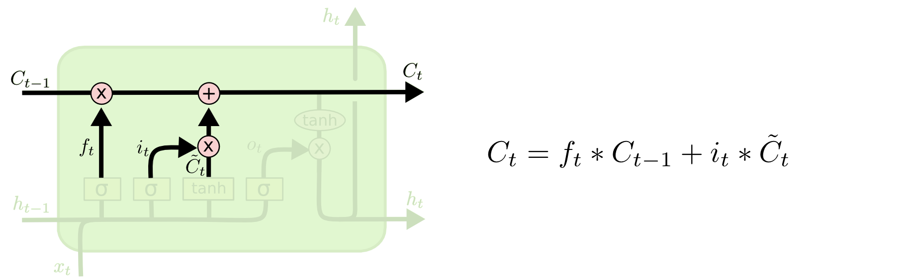
The cell state runs straight along the top of the diagram below with only two interactions: an elementwise multiplication (forgetting) and an elementwise addition (writing). No matrix multiplication, no repeated squashing.
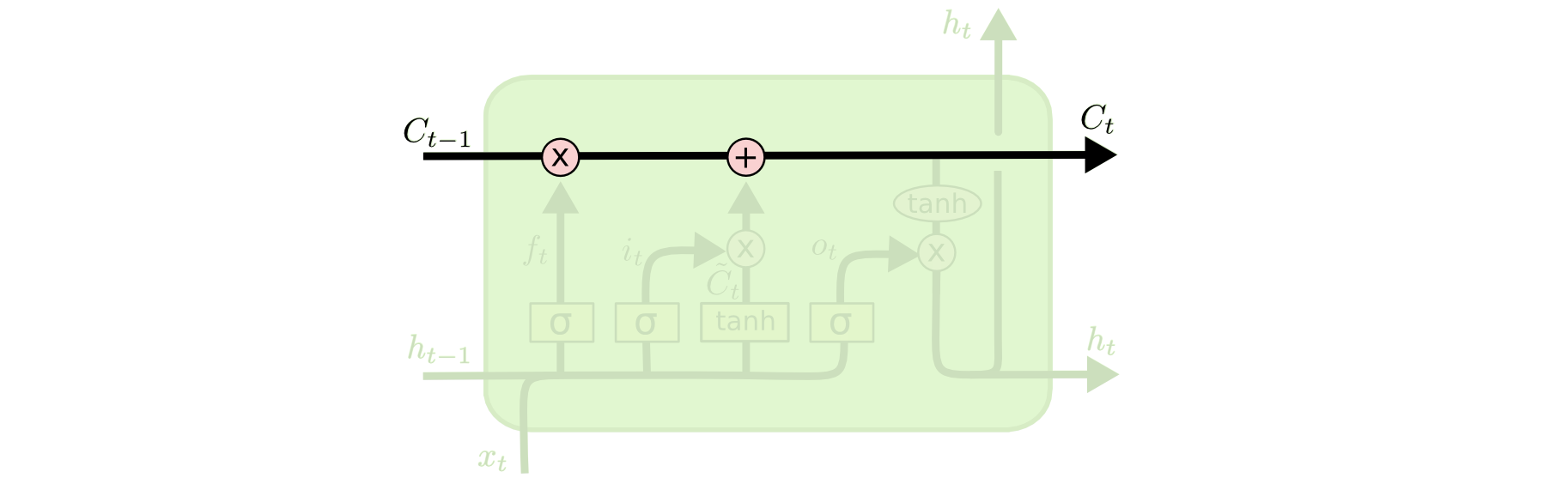 The cell state runs through the whole chain with only minor linear interactions — information can flow along it almost unchanged.
Source: colah.github.io
That additive update is the whole trick. If the forget gate stays near 1, then $c_t \approx c_{t-1} + \text{something}$, and the gradient flows backwards through the addition undiminished. The network can now choose to remember.
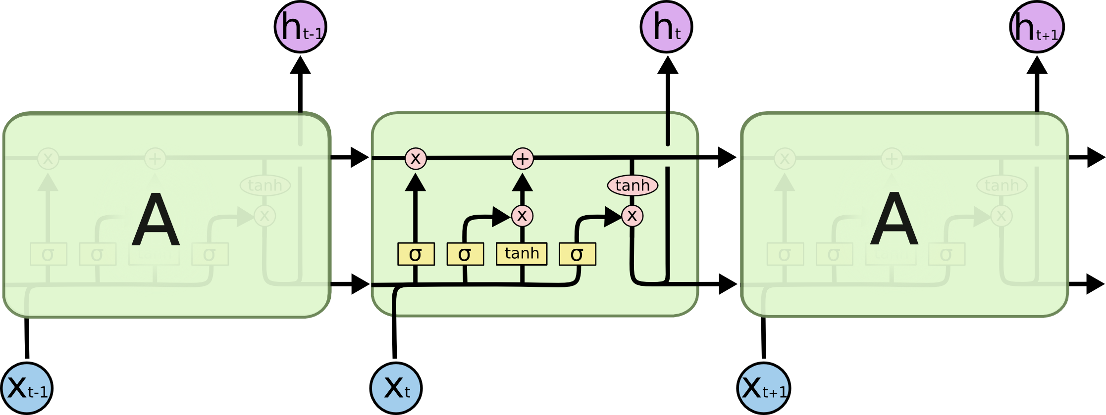 A full LSTM cell. The three sigmoid layers are the gates; each produces values in (0, 1) that act as valves on the information flow.
Source: colah.github.io
Redrawn with the names we will use in code, the same cell looks like this — notice how the red memory line crosses the whole diagram touching only a multiply and an add:

3. The Three Gates
A gate is a small neural layer with a sigmoid activation. Because $\sigma$ outputs values in $(0, 1)$, multiplying a vector by a gate output controls how much of it passes: 0 blocks everything, 1 lets everything through. All three gates look at the same two things — the current input $x_t$ and the previous hidden state $h_{t-1}$ — but they learn different weights and therefore different jobs.
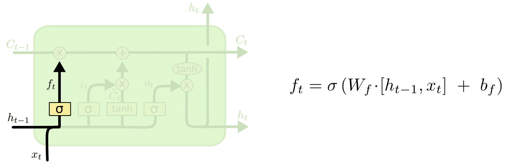
Forget gate — what should be erased from the cell state?
$$ f_t = \sigma\left(W_{if}\,x_t + b_{if} + W_{hf}\,h_{t-1} + b_{hf}\right) $$
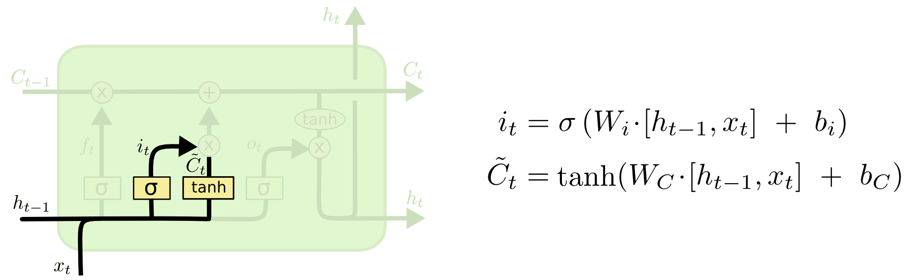
Input gate and candidate values — what new information should be written?
$$ i_t = \sigma\left(W_{ii}\,x_t + b_{ii} + W_{hi}\,h_{t-1} + b_{hi}\right) $$
$$ g_t = \tanh\left(W_{ig}\,x_t + b_{ig} + W_{hg}\,h_{t-1} + b_{hg}\right) $$
Cell state update — forget some of the old, add some of the new:
$$ c_t = f_t \odot c_{t-1} + i_t \odot g_t $$
Output gate — what part of the memory should be exposed right now?
$$ o_t = \sigma\left(W_{io}\,x_t + b_{io} + W_{ho}\,h_{t-1} + b_{ho}\right) $$
$$ h_t = o_t \odot \tanh(c_t) $$
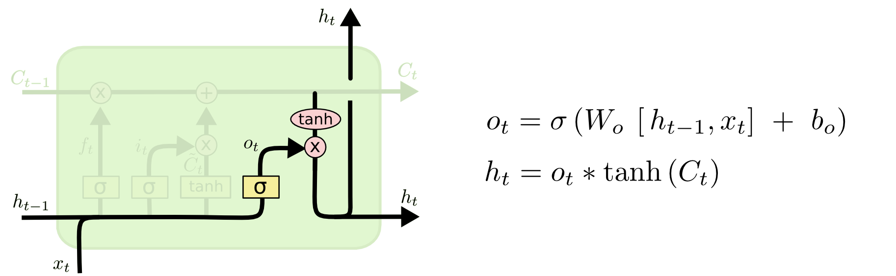 Source of all four diagrams: colah.github.io
Here $\odot$ is elementwise multiplication. Note that $c_t$ and $h_t$ are decoupled: the cell can hold a fact for a hundred steps while the output gate keeps it hidden until it becomes relevant.
Implementing an LSTM cell from scratch
The four gates are computed from the same two inputs, so PyTorch packs their weights into single matrices of shape (4 * hidden_size, ...) and splits the result into four chunks. The chunk order is i, f, g, o — worth remembering, because it differs from the order the equations are usually presented in.
import torch
import torch.nn as nn

torch.manual_seed(0)

input_size, hidden_size, seq_len = 3, 4, 5
x_seq = torch.randn(seq_len, input_size)

cell = nn.LSTMCell(input_size, hidden_size)

def manual_lstm_cell(x_t, h_prev, c_prev, cell):
    """One LSTM step written out by hand, borrowing PyTorch's weights."""
    gates = (x_t @ cell.weight_ih.T + cell.bias_ih
             + h_prev @ cell.weight_hh.T + cell.bias_hh)     # (batch, 4 * hidden)

    i, f, g, o = gates.chunk(4, dim=1)   # PyTorch packs the gates in this order
    i = torch.sigmoid(i)                 # input gate:  what to write
    f = torch.sigmoid(f)                 # forget gate: what to erase
    g = torch.tanh(g)                    # candidate:   the values to write
    o = torch.sigmoid(o)                 # output gate: what to expose

    c_t = f * c_prev + i * g             # the additive memory update
    h_t = o * torch.tanh(c_t)
    return h_t, c_t

h_m = torch.zeros(1, hidden_size)
c_m = torch.zeros(1, hidden_size)
h_p = torch.zeros(1, hidden_size)
c_p = torch.zeros(1, hidden_size)

for t in range(seq_len):
    x_t = x_seq[t].unsqueeze(0)
    h_m, c_m = manual_lstm_cell(x_t, h_m, c_m, cell)   # ours
    h_p, c_p = cell(x_t, (h_p, c_p))                   # PyTorch's

print('Manual  h_T:', h_m.detach().numpy().round(4))
print('PyTorch h_T:', h_p.detach().numpy().round(4))
print('Hidden match:', torch.allclose(h_m, h_p, atol=1e-6))
print('Cell match  :', torch.allclose(c_m, c_p, atol=1e-6))
Manual  h_T: [[-0.234   0.0802  0.1348 -0.3747]]
PyTorch h_T: [[-0.234   0.0802  0.1348 -0.3747]]
Hidden match: True
Cell match  : True
Inspecting the gates
Printing the gate values for a single step makes their role tangible. Values near 0 mean "block", values near 1 mean "pass".
gates = (x_seq[0].unsqueeze(0) @ cell.weight_ih.T + cell.bias_ih
         + torch.zeros(1, hidden_size) @ cell.weight_hh.T + cell.bias_hh)
i, f, g, o = gates.chunk(4, dim=1)

print('input  gate i:', torch.sigmoid(i).detach().numpy().round(3))
print('forget gate f:', torch.sigmoid(f).detach().numpy().round(3))
print('candidate  g:', torch.tanh(g).detach().numpy().round(3))
print('output gate o:', torch.sigmoid(o).detach().numpy().round(3))
input  gate i: [[0.446 0.129 0.527 0.541]]
forget gate f: [[0.183 0.545 0.314 0.602]]
candidate  g: [[ 0.431 -0.58  -0.37  -0.778]]
output gate o: [[0.874 0.19  0.442 0.528]]
4. LSTMs in PyTorch: nn.LSTM
nn.LSTM follows the same conventions as nn.RNN, with one difference: the state is a tuple (h0, c0) instead of a single tensor, and the layer returns (h_n, c_n) the same way.
- Input with
batch_first=True:(batch_size, seq_len, input_size) - State: a tuple of two tensors, each
(num_layers, batch_size, hidden_size) - Output
out:(batch_size, seq_len, hidden_size)— the hidden state at every step (never the cell state)
import torch.optim as optim
print('PyTorch version:', torch.__version__)

batch = torch.randn(2, 5, 3)
lstm = nn.LSTM(input_size=3, hidden_size=4, num_layers=1, batch_first=True)
out, (hn, cn) = lstm(batch)

print('input shape:', tuple(batch.shape))
print('out shape  :', tuple(out.shape))
print('hn shape   :', tuple(hn.shape))
print('cn shape   :', tuple(cn.shape))
print('out[:, -1, :] == hn[-1]:', torch.allclose(out[:, -1, :], hn[-1]))

# An LSTM has 4x the parameters of an RNN with the same hidden size - one set per gate
rnn = nn.RNN(input_size=3, hidden_size=4, batch_first=True)
print('RNN  params:', sum(p.numel() for p in rnn.parameters()))
print('LSTM params:', sum(p.numel() for p in lstm.parameters()))
PyTorch version: 2.13.0+cpu
input shape: (2, 5, 3)
out shape  : (2, 5, 4)
hn shape   : (1, 2, 4)
cn shape   : (1, 2, 4)
out[:, -1, :] == hn[-1]: True
RNN  params: 36
LSTM params: 144
5. A Task That Requires Long-Term Memory
To compare the architectures we need a task where the answer depends on something that happened long ago. Here is a clean one:
Each sequence starts with a marker, either $+1$ or $-1$. Everything after it is noise. The label is the sign of that first value.
A model that only looks at recent steps is reduced to guessing — it can score 50% and no better. To beat that, one bit of information has to survive from step 1 all the way to step $T$.
import numpy as np
from torch.utils.data import TensorDataset, DataLoader

def make_memory_dataset(n_samples, seq_len, seed=0):
    """A +/-1 marker in the first position, pure noise afterwards."""
    g = torch.Generator().manual_seed(seed)
    X = torch.rand(n_samples, seq_len, 1, generator=g) * 2 - 1     # noise in [-1, 1]
    marker = torch.randint(0, 2, (n_samples,), generator=g).float() * 2 - 1
    X[:, 0, 0] = marker                                            # overwrite step 1
    y = (X[:, 0, 0] > 0).float().unsqueeze(1)                      # label from step 1 only
    return X, y

SEQ_LEN = 60
X_train, y_train = make_memory_dataset(2000, SEQ_LEN, seed=0)
X_test, y_test = make_memory_dataset(1000, SEQ_LEN, seed=1)

train_loader = DataLoader(TensorDataset(X_train, y_train), batch_size=64, shuffle=True)
test_loader = DataLoader(TensorDataset(X_test, y_test), batch_size=256, shuffle=False)

print('X_train:', tuple(X_train.shape), 'y_train:', tuple(y_train.shape))
print('Class balance (fraction of 1s):', y_train.mean().item())
print('First sequence starts with:', X_train[0, :4, 0].numpy().round(3),
      '-> label', int(y_train[0].item()))
X_train: (2000, 60, 1) y_train: (2000, 1)
Class balance (fraction of 1s): 0.5130000114440918
First sequence starts with: [ 1.     0.536 -0.823 -0.736] -> label 1
6. Defining the Models
One class, with the recurrent layer chosen by name, so the only difference between the runs is the cell type. nn.LSTM, nn.GRU and nn.RNN are drop-in replacements for one another here, because we let PyTorch initialise the state to zeros and only read out.
The forget_bias argument will stay unused for now. We will need it shortly, and the reason why is the most useful thing in this lab.
The output is a single logit, and we use nn.BCEWithLogitsLoss, which folds a sigmoid into a numerically stable cross-entropy. (This is why the model does not end with nn.Sigmoid() — applying it twice would be a bug.)
def set_forget_gate_bias(lstm_layer, value=1.0):
    """PyTorch packs the LSTM biases as [i, f, g, o]; the second quarter is the forget gate."""
    for name, param in lstm_layer.named_parameters():
        if 'bias' in name:
            n = param.size(0)
            param.data[n // 4: n // 2].fill_(value)

class SequenceClassifier(nn.Module):
    def __init__(self, cell_type='lstm', input_size=1, hidden_size=32,
                 num_layers=1, forget_bias=None):
        super(SequenceClassifier, self).__init__()
        layer = {'lstm': nn.LSTM, 'rnn': nn.RNN, 'gru': nn.GRU}[cell_type]
        self.rnn = layer(input_size, hidden_size, num_layers, batch_first=True)
        if forget_bias is not None and cell_type == 'lstm':
            set_forget_gate_bias(self.rnn, forget_bias)
        self.fc = nn.Linear(hidden_size, 1)

    def forward(self, x):
        out, _ = self.rnn(x)             # works for RNN, GRU and LSTM alike
        return self.fc(out[:, -1, :])    # raw logit, no sigmoid here

torch.manual_seed(0)
lstm_model = SequenceClassifier('lstm')
rnn_model = SequenceClassifier('rnn')
print(lstm_model)
print('LSTM params:', sum(p.numel() for p in lstm_model.parameters()))
print('RNN  params:', sum(p.numel() for p in rnn_model.parameters()))
SequenceClassifier(
  (rnn): LSTM(1, 32, batch_first=True)
  (fc): Linear(in_features=32, out_features=1, bias=True)
)
LSTM params: 4513
RNN  params: 1153
7. The First Attempt
Train both identically and compare. Gradient clipping is included because it is standard practice for recurrent networks — it caps the gradient norm so a single exploding update cannot destroy the weights.
Before you run it: the LSTM has four times the parameters, a dedicated memory path, and was invented specifically for this problem. Predict the result.
device = torch.device('cuda' if torch.cuda.is_available() else 'cpu')
criterion = nn.BCEWithLogitsLoss()

def evaluate(model, loader):
    model.eval()
    correct = total = 0
    with torch.no_grad():
        for xb, yb in loader:
            xb, yb = xb.to(device), yb.to(device)
            pred = (torch.sigmoid(model(xb)) > 0.5).float()
            correct += (pred == yb).sum().item()
            total += yb.size(0)
    return 100 * correct / total

def train(model, num_epochs=15, lr=3e-3, verbose=True):
    model.to(device)
    optimizer = optim.Adam(model.parameters(), lr=lr)
    history = []
    for epoch in range(num_epochs):
        model.train()
        for xb, yb in train_loader:
            xb, yb = xb.to(device), yb.to(device)
            optimizer.zero_grad()
            loss = criterion(model(xb), yb)
            loss.backward()
            nn.utils.clip_grad_norm_(model.parameters(), 1.0)
            optimizer.step()
        acc = evaluate(model, test_loader)
        history.append(acc)
        if verbose and (epoch + 1) % 5 == 0:
            print(f'  epoch [{epoch+1}/{num_epochs}], test accuracy: {acc:.2f}%')
    return history

def run_seed(cell_type, seed, forget_bias=None, verbose=False):
    """One full training run from a given seed. The seed fixes both the weight
    initialisation and the order the batches are shuffled in."""
    torch.manual_seed(seed)
    model = SequenceClassifier(cell_type, forget_bias=forget_bias)
    return model, train(model, verbose=verbose)

print(f'Training LSTM on sequences of length {SEQ_LEN} (seed 0)...')
lstm_model, lstm_hist = run_seed('lstm', 0, verbose=True)
print(f'\nTraining vanilla RNN on sequences of length {SEQ_LEN} (seed 0)...')
rnn_model, rnn_hist = run_seed('rnn', 0, verbose=True)

print(f'\nFinal LSTM accuracy: {lstm_hist[-1]:.2f}%')
print(f'Final RNN  accuracy: {rnn_hist[-1]:.2f}%')
print('Chance level: 50.00%')
Training LSTM on sequences of length 60 (seed 0)...
epoch [5/15], test accuracy: 47.40%
epoch [10/15], test accuracy: 47.00%
  epoch [15/15], test accuracy: 49.20%

Training vanilla RNN on sequences of length 60 (seed 0)...
epoch [5/15], test accuracy: 47.40%
epoch [10/15], test accuracy: 47.20%
  epoch [15/15], test accuracy: 100.00%

Final LSTM accuracy: 49.20%
Final RNN  accuracy: 100.00%
Chance level: 50.00%
import matplotlib.pyplot as plt

plt.figure(figsize=(7, 4))
plt.plot(range(1, len(lstm_hist) + 1), lstm_hist, marker='o', label='LSTM')
plt.plot(range(1, len(rnn_hist) + 1), rnn_hist, marker='s', label='vanilla RNN')
plt.axhline(50, color='gray', linestyle=':', label='chance')
plt.xlabel('Epoch')
plt.ylabel('Test accuracy (%)')
plt.title(f'One seed, {SEQ_LEN} steps')
plt.legend()
plt.grid(alpha=0.3)
plt.show()

Whatever you just got, do not draw a conclusion from it yet.
That is not a figure of speech. This exact comparison was run twice while writing this lab, with identical hyperparameters, and produced opposite results — once the RNN reached 100% while the LSTM sat at chance, and once the reverse. The only difference was the order in which random numbers were drawn.
A single training run is one sample from a distribution. On this task the distribution turns out to be bimodal: a model either discovers how to carry the marker across 60 steps, or it never does and stays at 50%. There is very little in between. Averaging two such runs is meaningless; what you want to know is how often each architecture finds the solution.
So let's ask that question properly.
8. Run It Again, and Again
The same two architectures, five seeds each. What matters is not the mean accuracy — averaging a bimodal distribution produces a number no single run ever shows — but the solve rate: how many seeds got there at all.
This takes a few minutes. It is the most important cell in the lab.
SEEDS = [0, 1, 2, 3, 4]
SOLVED = 90        # above this we call the task solved; runs land near 100 or near 50

results = {'vanilla RNN': [rnn_hist[-1]], 'LSTM (default init)': [lstm_hist[-1]]}

for seed in SEEDS[1:]:                      # seed 0 was done in section 7
    _, h = run_seed('rnn', seed)
    results['vanilla RNN'].append(h[-1])
    _, h = run_seed('lstm', seed)
    results['LSTM (default init)'].append(h[-1])
    print(f'  seed {seed} done', flush=True)

def report(results):
    print(f'\n{"variant":22s} ' + ' '.join(f'{f"seed {s}":>8}' for s in SEEDS)
          + f' | {"solved":>7}')
    print('-' * (24 + 9 * len(SEEDS) + 10))
    for name, accs in results.items():
        solved = sum(a > SOLVED for a in accs)
        print(f'{name:22s} ' + ' '.join(f'{a:>8.1f}' for a in accs)
              + f' | {solved:>3}/{len(accs)}')

report(results)
seed 1 done
seed 2 done
seed 3 done
seed 4 done
variant                  seed 0   seed 1   seed 2   seed 3   seed 4 |  solved
-------------------------------------------------------------------------------
vanilla RNN               100.0    100.0     47.9     47.7     47.3 |   2/5
LSTM (default init)        49.2     49.3     50.2     50.4     47.5 |   0/5
fig, ax = plt.subplots(figsize=(8, 4))
for i, (name, accs) in enumerate(results.items()):
    ax.scatter([i] * len(accs), accs, s=90, alpha=0.75,
               color=['#4C72B0', '#C44E52'][i % 2])
ax.axhline(50, color='gray', linestyle=':', label='chance')
ax.axhline(SOLVED, color='#55A868', linestyle='--', label='solved')
ax.set_xticks(range(len(results)), list(results), fontsize=9)
ax.set_ylim(40, 105)
ax.set_ylabel('final test accuracy (%)')
ax.set_title('Every seed, plotted separately — note the gap in the middle')
ax.legend(fontsize=8)
ax.grid(alpha=0.3, axis='y')
plt.tight_layout()
plt.show()

Two facts survive the noise, and they are not the ones the textbook story predicts:
- The vanilla RNN sometimes solves it. Not reliably — but it can. If it learns $W_{hh} \approx 1$ on a single hidden unit, that unit becomes a running integrator carrying the marker forward almost unchanged. Vanishing gradients make that hard to find, not impossible to represent.
- The default LSTM essentially never solves it, across every seed tried. That is remarkably consistent for a task it was designed for.
The LSTM's failure being consistent is the useful clue. Bad luck is random; this is systematic. Something about the LSTM at initialisation is actively wrong for this problem.
9. Diagnosis: the Forget Gate Starts Half Closed
Look again at the cell state update:
$$ c_t = f_t \odot c_{t-1} + i_t \odot g_t $$
Memory survives one step multiplied by $f_t$, so over $T$ steps it survives multiplied by $\prod f_t$. Now ask what $f_t$ is at initialisation. PyTorch initialises the biases near zero and the weights small, so the pre-activation is near zero, and
$$ f_t = \sigma(\approx 0) \approx 0.5 $$
Halving the memory at every step means a half-life of about one step. After 60 steps the marker has been multiplied by roughly $0.5^{60} \approx 10^{-18}$. The LSTM does not start with a memory highway — it starts with a memory shredder, and it has to learn its way out of that before it can begin learning the task.
Let's measure it rather than assume it.
import math

def mean_forget_gate(forget_bias=None, hidden_size=32, steps=40, seed=0):
    """Average forget-gate value of an untrained LSTM, and the implied memory half-life."""
    torch.manual_seed(seed)
    layer = nn.LSTM(1, hidden_size, batch_first=True)
    if forget_bias is not None:
        set_forget_gate_bias(layer, forget_bias)

    x = torch.randn(1, steps, 1)
    h = torch.zeros(1, hidden_size)
    c = torch.zeros(1, hidden_size)
    values = []
    with torch.no_grad():
        for t in range(steps):
            gates = (x[0, t].unsqueeze(0) @ layer.weight_ih_l0.T + layer.bias_ih_l0
                     + h @ layer.weight_hh_l0.T + layer.bias_hh_l0)
            i, f, g, o = gates.chunk(4, dim=1)
            i, f, g, o = torch.sigmoid(i), torch.sigmoid(f), torch.tanh(g), torch.sigmoid(o)
            c = f * c + i * g
            h = o * torch.tanh(c)
            values.append(f.mean().item())
    mean_f = sum(values) / len(values)
    half_life = math.log(0.5) / math.log(mean_f) if mean_f < 1 else float('inf')
    return mean_f, half_life

print(f'{"forget bias":>12} | {"mean f":>7} | {"half-life":>10} | {"memory left after 60 steps":>26}')
print('-' * 68)
for bias in [None, 1.0, 3.0]:
    mean_f, half_life = mean_forget_gate(bias)
    label = 'default' if bias is None else f'{bias:.0f}'
    print(f'{label:>12} | {mean_f:>7.3f} | {half_life:>7.1f} st | {mean_f ** 60:>26.2e}')
 forget bias |  mean f |  half-life | memory left after 60 steps
--------------------------------------------------------------------
     default |   0.486 |     1.0 st |                   1.49e-19
           1 |   0.876 |     5.2 st |                   3.62e-04
           3 |   0.997 |   256.7 st |                   8.50e-01
There it is, and it is deterministic — no seeds, no variance, just the arithmetic of the initialisation. At default settings the forget gate averages about 0.5 and the memory half-life is one step. Setting the forget-gate bias to 1 pushes the gate to roughly 0.88 and the half-life to about five steps; a bias of 3 puts it above 0.99, with a half-life of a couple of hundred steps.
This is why the forget-bias trick exists, and why it appears in every serious LSTM implementation. It is not a micro-optimisation.
10. Measuring Gradient Flow
In Lab 10 we measured how much gradient reaches the first time step. Running the same probe on the LSTM — at several forget-bias settings — turns the argument above into numbers.
These are untrained networks, so this measures what each architecture offers before learning, which is exactly the question raised by section 8.
def gradient_reaching_first_step(cell_type, T, hidden_size=32, seed=0, forget_bias=None):
    """Norm of d(sum of final hidden state) / d(x_1) for a sequence of length T."""
    torch.manual_seed(seed)
    layer = {'rnn': nn.RNN, 'lstm': nn.LSTM, 'gru': nn.GRU}[cell_type]
    probe = layer(input_size=1, hidden_size=hidden_size, batch_first=True)
    if forget_bias is not None and cell_type == 'lstm':
        set_forget_gate_bias(probe, forget_bias)
    x = torch.randn(1, T, 1, requires_grad=True)
    out, _ = probe(x)
    out[:, -1, :].sum().backward()
    return x.grad[0, 0].norm().item()

lengths = [5, 10, 20, 40, 80, 160]
series = {
    'RNN': [gradient_reaching_first_step('rnn', T) for T in lengths],
    'LSTM (default)': [gradient_reaching_first_step('lstm', T) for T in lengths],
    'LSTM (bias 1)': [gradient_reaching_first_step('lstm', T, forget_bias=1.0) for T in lengths],
    'LSTM (bias 3)': [gradient_reaching_first_step('lstm', T, forget_bias=3.0) for T in lengths],
}

header = f'{"T":>5} | ' + ' | '.join(f'{name:>14}' for name in series)
print(header)
print('-' * len(header))
for i, T in enumerate(lengths):
    print(f'{T:>5} | ' + ' | '.join(f'{series[name][i]:>14.2e}' for name in series))

plt.figure(figsize=(7, 4.5))
for name, values in series.items():
    plt.semilogy(lengths, values, marker='o', label=name)
plt.xlabel('sequence length T')
plt.ylabel('gradient norm at the first step (log scale)')
plt.title('How far back the learning signal reaches')
plt.legend(fontsize=9)
plt.grid(alpha=0.3, which='both')
plt.show()
    T |            RNN | LSTM (default) |  LSTM (bias 1) |  LSTM (bias 3)
-------------------------------------------------------------------------
    5 |       5.52e-02 |       8.23e-03 |       9.11e-02 |       1.49e-01
   10 |       5.03e-03 |       2.41e-04 |       4.92e-02 |       1.20e-01
   20 |       3.67e-05 |       3.04e-06 |       3.52e-03 |       7.44e-02
   40 |       1.75e-09 |       7.88e-10 |       2.84e-02 |       7.07e-02
   80 |       4.26e-18 |       1.27e-17 |       7.58e-03 |       1.68e-01
  160 |       5.28e-36 |       7.90e-33 |       2.14e-04 |       8.91e-03

Read the table carefully, because it contains the correction to a very common claim.
A default-initialised LSTM is not meaningfully better than a vanilla RNN here — at short lengths it is worse. Both collapse to numbers no optimizer can use. Open the forget gate, though, and the gradient at 160 steps improves by roughly thirty orders of magnitude.
So the honest statement is not "LSTMs preserve gradients". It is:
An LSTM can preserve gradients, because the additive cell-state path makes it possible. Whether it does is decided by the forget gate — and at default initialisation, the forget gate says no.
Gating buys controllable memory. The initialisation decides where that control starts.
11. The One-Line Fix
Now retrain the LSTM with the forget-gate bias set to 1, changing nothing else — and evaluate it the way section 8 established, across every seed.
torch.manual_seed(0)
preview = SequenceClassifier('lstm', forget_bias=1.0)
print('Forget-gate quarter of bias_ih_l0:',
      preview.rnn.bias_ih_l0.data[32:64][:8].numpy().round(2), '...')

results['LSTM (forget bias 1)'] = []
for seed in SEEDS:
    model, h = run_seed('lstm', seed, forget_bias=1.0)
    results['LSTM (forget bias 1)'].append(h[-1])
    if seed == 0:
        lstm_fixed = model                  # kept for the gate animation below
    print(f'  seed {seed}: {h[-1]:.2f}%', flush=True)

report(results)
Forget-gate quarter of bias_ih_l0: [1. 1. 1. 1. 1. 1. 1. 1.] ...
seed 0: 100.00%
seed 1: 95.20%
seed 2: 100.00%
seed 3: 97.30%
seed 4: 100.00%
variant                  seed 0   seed 1   seed 2   seed 3   seed 4 |  solved
-------------------------------------------------------------------------------
vanilla RNN               100.0    100.0     47.9     47.7     47.3 |   2/5
LSTM (default init)        49.2     49.3     50.2     50.4     47.5 |   0/5
LSTM (forget bias 1)      100.0     95.2    100.0     97.3    100.0 |   5/5
fig, ax = plt.subplots(figsize=(9, 4.2))
colors = ['#C44E52', '#8172B3', '#55A868']
for i, (name, accs) in enumerate(results.items()):
    ax.scatter([i] * len(accs), accs, s=100, alpha=0.8, color=colors[i % len(colors)])
    ax.text(i, 103, f'{sum(a > SOLVED for a in accs)}/{len(accs)}',
            ha='center', fontsize=10, weight='bold')
ax.axhline(50, color='gray', linestyle=':', label='chance')
ax.axhline(SOLVED, color='#55A868', linestyle='--', label='solved')
ax.set_xticks(range(len(results)), list(results), fontsize=9)
ax.set_ylim(40, 108)
ax.set_ylabel('final test accuracy (%)')
ax.set_title('Solve rate across seeds — the number above each column is what matters')
ax.legend(fontsize=8, loc='center right')
ax.grid(alpha=0.3, axis='y')
plt.tight_layout()
plt.show()

That is the result the lab was after, and it only became visible once every configuration was run several times:
- Default LSTM: almost never solves the task. Consistent, and explained by the half-life table.
- Vanilla RNN: sometimes solves it. Unreliable, because it has to discover a near-identity recurrence through vanishing gradients.
- LSTM with the forget gate opened: solves it most of the time.
One line of initialisation moved the LSTM from the bottom of that list to the top. And had we judged any of them on a single run, we could have concluded almost anything — which is the second lesson, and the more broadly useful one.
Watching the trained gates at work
Now that we have an LSTM that learned the task, we can run one sequence through it step by step and watch what the gates actually do. This is the payoff of understanding the equations: gate values are just tensors, and you can look at them.
Two things to watch:
- the forget gate staying high on the units that carry the answer, keeping them alive
- the cell state locking in a value during the first few steps and then barely moving for the remaining 50-odd steps of noise
from matplotlib import animation
import os

os.makedirs('Misc', exist_ok=True)

def save_animation(ani, filename, fps=8, dpi=80):
    """Render an animation to a GIF under Misc/ and report where it went."""
    path = os.path.join('Misc', filename)
    ani.save(path, writer='pillow', fps=fps, dpi=dpi)
    print(f'saved {path}  ({os.path.getsize(path) / 1e6:.1f} MB)')
    return path

def gate_trace(model, sequence):
    """Replay a sequence through a trained nn.LSTM one step at a time, recording the gates."""
    lstm = model.rnn
    W_ih, W_hh = lstm.weight_ih_l0, lstm.weight_hh_l0
    b_ih, b_hh = lstm.bias_ih_l0, lstm.bias_hh_l0
    H = lstm.hidden_size

    h = torch.zeros(1, H, device=sequence.device)
    c = torch.zeros(1, H, device=sequence.device)
    trace = {'i': [], 'f': [], 'o': [], 'c': []}

    with torch.no_grad():
        for t in range(sequence.size(0)):
            x_t = sequence[t].unsqueeze(0)
            gates = x_t @ W_ih.T + b_ih + h @ W_hh.T + b_hh
            i, f, g, o = gates.chunk(4, dim=1)
            i, f, g, o = torch.sigmoid(i), torch.sigmoid(f), torch.tanh(g), torch.sigmoid(o)
            c = f * c + i * g
            h = o * torch.tanh(c)
            for key, val in zip(['i', 'f', 'o', 'c'], [i, f, o, c]):
                trace[key].append(val.squeeze(0).cpu().numpy().copy())
    return {k: np.stack(v) for k, v in trace.items()}

sample = X_test[0].to(device)                  # (SEQ_LEN, 1)
tr = gate_trace(lstm_fixed, sample)
print(f'First value of this sequence: {sample[0, 0].item():.3f}'
      f'  ->  true label {int(y_test[0].item())}')
print(f'Mean forget-gate value after training: {tr["f"].mean():.3f}')
First value of this sequence: -1.000  ->  true label 0
Mean forget-gate value after training: 0.904
H = tr['f'].shape[1]
fig, axes = plt.subplots(4, 1, figsize=(9, 6), sharex=True)
titles = [('f', 'forget gate  (1 = keep the memory)', '#DD8452', (0, 1)),
          ('i', 'input gate  (1 = write new information)', '#CCB974', (0, 1)),
          ('o', 'output gate  (1 = expose the memory)', '#8172B3', (0, 1)),
          ('c', 'cell state  (the long-term memory itself)', '#C44E52', (-2, 2))]

bars = []
for ax, (key, title, color, ylim) in zip(axes, titles):
    ax.set_title(title, fontsize=10, loc='left')
    ax.set_ylim(*ylim)
    ax.axhline(0, color='gray', lw=0.6)
    bars.append(ax.bar(range(H), [0] * H, color=color))
axes[-1].set_xlabel('hidden unit')

def update(t):
    for (key, _, _, _), bar_set in zip(titles, bars):
        for bar, v in zip(bar_set, tr[key][t]):
            bar.set_height(v)
    fig.suptitle(f'step {t + 1} of {SEQ_LEN}'
                 + ('   <- the informative step' if t == 0 else '   (pure noise)'))
    return [b for bar_set in bars for b in bar_set]

fig.tight_layout()
ani = animation.FuncAnimation(fig, update, frames=SEQ_LEN, interval=140, blit=False)
plt.close(fig)
save_animation(ani, 'lab11_gates.gif', fps=7)
saved Misc\lab11_gates.gif (1.1 MB)
'Misc\\lab11_gates.gif'
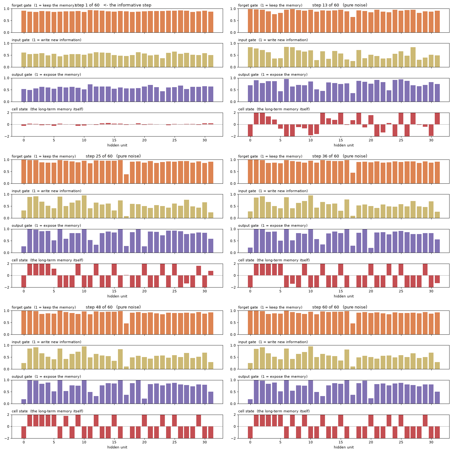 The trained gates at work: the forget gate holds the answer while 59 steps of noise go past.
12. GRU: a Lighter Alternative
The Gated Recurrent Unit simplifies the LSTM: it merges the cell state and hidden state into one, and merges the forget and input gates into a single update gate. Two gates instead of three, roughly 25% fewer parameters, and often the same accuracy.
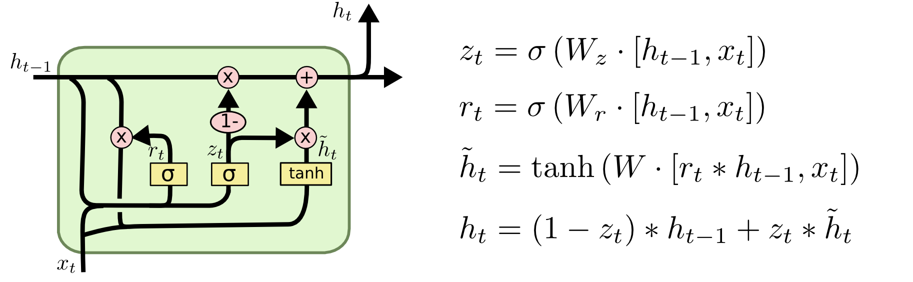 The GRU cell: an update gate decides how much of the old state to keep versus overwrite, and a reset gate controls how much history feeds the candidate.
Source: colah.github.io
$$ z_t = \sigma\left(W_{iz}\,x_t + W_{hz}\,h_{t-1} + b_z\right) \quad \text{(update gate)} $$
$$ r_t = \sigma\left(W_{ir}\,x_t + W_{hr}\,h_{t-1} + b_r\right) \quad \text{(reset gate)} $$
$$ n_t = \tanh\left(W_{in}\,x_t + r_t \odot (W_{hn}\,h_{t-1}) + b_n\right) $$
$$ h_t = (1 - z_t) \odot n_t + z_t \odot h_{t-1} $$
Look at that last line with section 9 in mind. Memory is retained in proportion to $z_t$, and at initialisation $z_t = \sigma(\approx 0) \approx 0.5$ — the GRU has exactly the same problem, for exactly the same reason. Predict its solve rate before running the cell.
results['GRU (default init)'] = []
for seed in SEEDS:
    _, h = run_seed('gru', seed)
    results['GRU (default init)'].append(h[-1])

report(results)
print(f'\nGRU params : {sum(p.numel() for p in SequenceClassifier("gru").parameters()):,}')
print(f'LSTM params: {sum(p.numel() for p in SequenceClassifier("lstm").parameters()):,}')
variant                  seed 0   seed 1   seed 2   seed 3   seed 4 |  solved
-------------------------------------------------------------------------------
vanilla RNN               100.0    100.0     47.9     47.7     47.3 |   2/5
LSTM (default init)        49.2     49.3     50.2     50.4     47.5 |   0/5
LSTM (forget bias 1)      100.0     95.2    100.0     97.3    100.0 |   5/5
GRU (default init)         50.0     47.7     47.9     51.0     51.7 |   0/5

GRU params : 3,393
LSTM params: 4,513
The GRU has the same fix. PyTorch packs the GRU weights in the order $r, z, n$, so the second quarter of
bias_ih_l0is the update gate. Setting it positive biases the cell towards keeping its state, exactly asset_forget_gate_biasdoes for the LSTM. Try it — it is in the experiment list below.
Which should you use? There is no universal winner. Start with an LSTM or GRU rather than a vanilla RNN, initialise the retention gate open, try both if the task matters, and prefer the GRU when data or compute is tight. For very long sequences, attention-based models — the subject of Lab 14 — have largely replaced both.
13. Experiment: Try Different Architectures and Hyperparameters
You can experiment with:
- Adding seeds 5 to 9 to
SEEDSand watching the solve rates settle. How many runs before the ordering stops changing? That number is worth knowing before you trust any comparison. - Applying the same trick to the GRU's update gate (second quarter of
bias_ih_l0) and re-measuring its solve rate - Trying
forget_bias=3.0instead of 1.0, and checking the result against the half-life table in section 9 - Sweeping
SEQ_LENover 20, 60, 150 and 300 — with the multi-seed protocol, since single runs at long lengths are especially unreliable. Section 9's table predicts which biases should survive which lengths; make the prediction first. - Stacking layers with
num_layers=2, dropout=0.2 - Setting
bidirectional=True(rememberhidden_size * 2in the finalnn.Linear) — this makes the task trivial, since the backward pass starts at the informative step - Removing
clip_grad_norm_and watching the vanilla RNN's training for instability
Try modifying the model definition or training loop above and observe how the performance changes.
14. Conclusion
In this lab you learned how LSTMs solve the problem that limits vanilla RNNs — and, more usefully, that the solution is conditional. The cell state provides an additive path along which information and gradient can travel far, and three learned gates decide what is erased, written and exposed. Whether that path is open at the start is a matter of initialisation, and by default it is not.
Key takeaways:
- The additive update $c_t = f_t \odot c_{t-1} + i_t \odot g_t$ is what makes long memory possible.
- A gate is a sigmoid used as a valve. At initialisation every gate sits near 0.5.
- A forget gate at 0.5 gives a memory half-life of one step, so a default LSTM forgets faster than a tanh RNN — and consistently fails this task.
- Initialising the forget-gate bias to 1 improved the gradient reaching step 1 of a 160-step sequence by about thirty orders of magnitude, and took the solve rate from near zero to most seeds.
- The GRU's update gate has the same issue and the same fix.
- A vanilla RNN is more capable than folklore suggests; it fails at finding long-range solutions reliably, not at representing them.
- Judge a stochastic method by its solve rate over several seeds, never by one run. Two single runs of this comparison produced opposite conclusions while this lab was being written.
The next lab moves from sequences back to images, and shows how to reuse a network someone else already trained instead of starting from random weights.