Lab 16: Generative Adversarial Networks (GANs)¶

The VAE in Lab 15 generated digits by reconstructing them, and its samples came out slightly blurry. That is not a bug you can tune away: when the loss is "how far is this pixel from the target", the safest prediction is an average, and an average of many digits is a blur.

GANs replace that hand-written loss with a second network trained to spot fakes. There is no pixel distance anywhere — the generator's only instruction is fool the critic.

We will cover the following topics:

The adversarial game, and the minimax objective behind it
Building a generator and a discriminator, and training them together
Reading GAN training curves, which look nothing like normal ones
Watching samples improve, epoch by epoch
Mode collapse and the other ways GAN training fails
The stability tricks that make it work in practice

1. Two Networks, One Game¶

A GAN is two networks with opposing objectives:

The generator $G$ turns a random vector $z$ into a fake image. It never sees real data.
The discriminator $D$ receives real and fake images and outputs the probability that the input is real.

They are trained on the same objective, in opposite directions:

$$ \min_G \max_D \; \mathbb{E}_{x \sim p_{\text{data}}}\left[\log D(x)\right] + \mathbb{E}_{z \sim p_z}\left[\log\left(1 - D(G(z))\right)\right] $$

$D$ wants to push the first term up (recognise real data) and the second term up (reject fakes). $G$ wants only to push the second term down. At the theoretical optimum $G$ reproduces the data distribution exactly and $D$ is reduced to guessing, outputting 0.5 everywhere.

The essential difference from every other model in these labs: the loss function is itself being learned. As $G$ improves, $D$ gets harder, which pushes $G$ further. Nobody ever specified what a digit should look like.

One practical amendment¶

As written, $G$ minimises $\log(1 - D(G(z)))$. Early in training $D$ rejects everything easily, that term saturates, and $G$ receives almost no gradient precisely when it needs the most.

So in practice $G$ maximises $\log D(G(z))$ instead — the "non-saturating" loss. Same fixed point, much stronger gradient when the generator is losing. In code this is just a binary cross-entropy against the label "real":

g_loss = criterion(D(fake), real_labels)   # G wants D to call its fakes real

In [1]:

Copied!





import torch
import torch.nn as nn
import torch.optim as optim
import numpy as np
import matplotlib.pyplot as plt
from torch.utils.data import DataLoader
from torchvision import datasets, transforms

torch.manual_seed(42)
np.random.seed(42)
device = torch.device('cuda' if torch.cuda.is_available() else 'cpu')
print('PyTorch version:', torch.__version__, '| device:', device)
if device.type == 'cpu':
    print('Note: this lab trains two networks at once. On CPU, reduce EPOCHS below.')

# Scale pixels to [-1, 1] to match the generator's tanh output
tf = transforms.Compose([
    transforms.ToTensor(),
    transforms.Normalize((0.5,), (0.5,)),
])
train_set = datasets.MNIST(root='./data', train=True, download=True, transform=tf)
train_loader = DataLoader(train_set, batch_size=128, shuffle=True, drop_last=True)
print(f'{len(train_set)} training images')
import torch
import torch.nn as nn
import torch.optim as optim
import numpy as np
import matplotlib.pyplot as plt
from torch.utils.data import DataLoader
from torchvision import datasets, transforms

torch.manual_seed(42)
np.random.seed(42)
device = torch.device('cuda' if torch.cuda.is_available() else 'cpu')
print('PyTorch version:', torch.__version__, '| device:', device)
if device.type == 'cpu':
    print('Note: this lab trains two networks at once. On CPU, reduce EPOCHS below.')

# Scale pixels to [-1, 1] to match the generator's tanh output
tf = transforms.Compose([
    transforms.ToTensor(),
    transforms.Normalize((0.5,), (0.5,)),
])
train_set = datasets.MNIST(root='./data', train=True, download=True, transform=tf)
train_loader = DataLoader(train_set, batch_size=128, shuffle=True, drop_last=True)
print(f'{len(train_set)} training images')

PyTorch version: 2.13.0+cpu | device: cpu
Note: this lab trains two networks at once. On CPU, reduce EPOCHS below.
60000 training images

2. The Two Networks¶

Both are small MLPs. The details that matter are at the boundaries:

The generator ends in tanh, so its output lives in $[-1, 1]$ — the same range we just normalised the real images to. A mismatch here makes the discriminator's job trivial and training collapses immediately.
The discriminator ends in a single logit, and we use BCEWithLogitsLoss.
Both use LeakyReLU. A dying ReLU in the discriminator kills the generator's gradient too, and the generator has no other teacher.

In [2]:

Copied!





LATENT_DIM = 64

class Generator(nn.Module):
    def __init__(self, latent_dim=LATENT_DIM, hidden=256):
        super(Generator, self).__init__()
        self.net = nn.Sequential(
            nn.Linear(latent_dim, hidden), nn.BatchNorm1d(hidden), nn.LeakyReLU(0.2),
            nn.Linear(hidden, hidden * 2), nn.BatchNorm1d(hidden * 2), nn.LeakyReLU(0.2),
            nn.Linear(hidden * 2, 784),
            nn.Tanh(),                       # matches the [-1, 1] data range
        )

    def forward(self, z):
        return self.net(z).view(-1, 1, 28, 28)

class Discriminator(nn.Module):
    def __init__(self, hidden=256):
        super(Discriminator, self).__init__()
        self.net = nn.Sequential(
            nn.Linear(784, hidden * 2), nn.LeakyReLU(0.2), nn.Dropout(0.3),
            nn.Linear(hidden * 2, hidden), nn.LeakyReLU(0.2), nn.Dropout(0.3),
            nn.Linear(hidden, 1),            # a single logit, no sigmoid
        )

    def forward(self, x):
        return self.net(x.view(x.size(0), -1))

G = Generator().to(device)
D = Discriminator().to(device)
print(f'Generator    : {sum(p.numel() for p in G.parameters()):,} parameters')
print(f'Discriminator: {sum(p.numel() for p in D.parameters()):,} parameters')
LATENT_DIM = 64

class Generator(nn.Module):
    def __init__(self, latent_dim=LATENT_DIM, hidden=256):
        super(Generator, self).__init__()
        self.net = nn.Sequential(
            nn.Linear(latent_dim, hidden), nn.BatchNorm1d(hidden), nn.LeakyReLU(0.2),
            nn.Linear(hidden, hidden * 2), nn.BatchNorm1d(hidden * 2), nn.LeakyReLU(0.2),
            nn.Linear(hidden * 2, 784),
            nn.Tanh(),                       # matches the [-1, 1] data range
        )

    def forward(self, z):
        return self.net(z).view(-1, 1, 28, 28)

class Discriminator(nn.Module):
    def __init__(self, hidden=256):
        super(Discriminator, self).__init__()
        self.net = nn.Sequential(
            nn.Linear(784, hidden * 2), nn.LeakyReLU(0.2), nn.Dropout(0.3),
            nn.Linear(hidden * 2, hidden), nn.LeakyReLU(0.2), nn.Dropout(0.3),
            nn.Linear(hidden, 1),            # a single logit, no sigmoid
        )

    def forward(self, x):
        return self.net(x.view(x.size(0), -1))

G = Generator().to(device)
D = Discriminator().to(device)
print(f'Generator    : {sum(p.numel() for p in G.parameters()):,} parameters')
print(f'Discriminator: {sum(p.numel() for p in D.parameters()):,} parameters')

Generator    : 551,952 parameters
Discriminator: 533,505 parameters

In [3]:

Copied!





# What an untrained generator produces
G.eval()
with torch.no_grad():
    noise = torch.randn(8, LATENT_DIM, device=device)
    fakes = G(noise).cpu()

fig, axes = plt.subplots(1, 8, figsize=(10, 1.6))
for ax, img in zip(axes, fakes):
    ax.imshow(img[0], cmap='gray', vmin=-1, vmax=1); ax.axis('off')
fig.suptitle('Before training: the generator is a random function', fontsize=10)
plt.tight_layout()
plt.show()
# What an untrained generator produces
G.eval()
with torch.no_grad():
    noise = torch.randn(8, LATENT_DIM, device=device)
    fakes = G(noise).cpu()

fig, axes = plt.subplots(1, 8, figsize=(10, 1.6))
for ax, img in zip(axes, fakes):
    ax.imshow(img[0], cmap='gray', vmin=-1, vmax=1); ax.axis('off')
fig.suptitle('Before training: the generator is a random function', fontsize=10)
plt.tight_layout()
plt.show()

No description has been provided for this image

3. The Training Loop¶

Each batch takes two steps.

Step 1 — train $D$. Show it real images labelled 1 and fake images labelled 0, and update it. Note the .detach() on the fakes: without it, the discriminator's backward pass would also compute gradients through the generator, which we do not want here.

Step 2 — train $G$. Generate fresh fakes, run them through $D$, and update $G$ as if the label were 1. Only $G$'s optimizer steps, so $D$ is unaffected.

Two small stabilisers are included, both standard:

One-sided label smoothing: use 0.9 rather than 1.0 for real images. An over-confident discriminator produces flat gradients.
Separate Adam optimizers with betas=(0.5, 0.999). The lowered momentum is a DCGAN-paper recommendation and it genuinely helps.

In [4]:

Copied!





criterion = nn.BCEWithLogitsLoss()
opt_G = optim.Adam(G.parameters(), lr=2e-4, betas=(0.5, 0.999))
opt_D = optim.Adam(D.parameters(), lr=2e-4, betas=(0.5, 0.999))

EPOCHS = 30                     # drop to 8-10 if you are on CPU and impatient
REAL_LABEL, FAKE_LABEL = 0.9, 0.0     # one-sided label smoothing

# A fixed noise vector, so every epoch's samples are directly comparable
fixed_noise = torch.randn(64, LATENT_DIM, device=device)

history = {'d_loss': [], 'g_loss': [], 'd_real': [], 'd_fake': []}
snapshots = []

for epoch in range(EPOCHS):
    G.train(); D.train()
    sums = np.zeros(4)
    batches = 0

    for real, _ in train_loader:
        real = real.to(device)
        batch = real.size(0)
        ones = torch.full((batch, 1), REAL_LABEL, device=device)
        zeros = torch.full((batch, 1), FAKE_LABEL, device=device)

        # --- step 1: the discriminator ---
        z = torch.randn(batch, LATENT_DIM, device=device)
        fake = G(z)
        d_real_out = D(real)
        d_fake_out = D(fake.detach())            # detach: do not touch G here
        d_loss = criterion(d_real_out, ones) + criterion(d_fake_out, zeros)

        opt_D.zero_grad()
        d_loss.backward()
        opt_D.step()

        # --- step 2: the generator ---
        z = torch.randn(batch, LATENT_DIM, device=device)
        fake = G(z)
        g_loss = criterion(D(fake), torch.ones(batch, 1, device=device))   # "call these real"

        opt_G.zero_grad()
        g_loss.backward()
        opt_G.step()

        sums += [d_loss.item(), g_loss.item(),
                 torch.sigmoid(d_real_out).mean().item(),
                 torch.sigmoid(d_fake_out).mean().item()]
        batches += 1

    for key, value in zip(['d_loss', 'g_loss', 'd_real', 'd_fake'], sums / batches):
        history[key].append(value)

    G.eval()
    with torch.no_grad():
        snapshots.append(G(fixed_noise).cpu().numpy())

    print(f'Epoch [{epoch+1}/{EPOCHS}]  D loss {history["d_loss"][-1]:.3f}  '
          f'G loss {history["g_loss"][-1]:.3f}  '
          f'D(real) {history["d_real"][-1]:.3f}  D(fake) {history["d_fake"][-1]:.3f}')
criterion = nn.BCEWithLogitsLoss()
opt_G = optim.Adam(G.parameters(), lr=2e-4, betas=(0.5, 0.999))
opt_D = optim.Adam(D.parameters(), lr=2e-4, betas=(0.5, 0.999))

EPOCHS = 30                     # drop to 8-10 if you are on CPU and impatient
REAL_LABEL, FAKE_LABEL = 0.9, 0.0     # one-sided label smoothing

# A fixed noise vector, so every epoch's samples are directly comparable
fixed_noise = torch.randn(64, LATENT_DIM, device=device)

history = {'d_loss': [], 'g_loss': [], 'd_real': [], 'd_fake': []}
snapshots = []

for epoch in range(EPOCHS):
    G.train(); D.train()
    sums = np.zeros(4)
    batches = 0

    for real, _ in train_loader:
        real = real.to(device)
        batch = real.size(0)
        ones = torch.full((batch, 1), REAL_LABEL, device=device)
        zeros = torch.full((batch, 1), FAKE_LABEL, device=device)

        # --- step 1: the discriminator ---
        z = torch.randn(batch, LATENT_DIM, device=device)
        fake = G(z)
        d_real_out = D(real)
        d_fake_out = D(fake.detach())            # detach: do not touch G here
        d_loss = criterion(d_real_out, ones) + criterion(d_fake_out, zeros)

        opt_D.zero_grad()
        d_loss.backward()
        opt_D.step()

        # --- step 2: the generator ---
        z = torch.randn(batch, LATENT_DIM, device=device)
        fake = G(z)
        g_loss = criterion(D(fake), torch.ones(batch, 1, device=device))   # "call these real"

        opt_G.zero_grad()
        g_loss.backward()
        opt_G.step()

        sums += [d_loss.item(), g_loss.item(),
                 torch.sigmoid(d_real_out).mean().item(),
                 torch.sigmoid(d_fake_out).mean().item()]
        batches += 1

    for key, value in zip(['d_loss', 'g_loss', 'd_real', 'd_fake'], sums / batches):
        history[key].append(value)

    G.eval()
    with torch.no_grad():
        snapshots.append(G(fixed_noise).cpu().numpy())

    print(f'Epoch [{epoch+1}/{EPOCHS}]  D loss {history["d_loss"][-1]:.3f}  '
          f'G loss {history["g_loss"][-1]:.3f}  '
          f'D(real) {history["d_real"][-1]:.3f}  D(fake) {history["d_fake"][-1]:.3f}')

Epoch [1/30]  D loss 1.236  G loss 0.988  D(real) 0.591  D(fake) 0.460

Epoch [2/30]  D loss 1.171  G loss 1.159  D(real) 0.575  D(fake) 0.389

Epoch [3/30]  D loss 1.151  G loss 1.234  D(real) 0.575  D(fake) 0.363

Epoch [4/30]  D loss 1.127  G loss 1.275  D(real) 0.578  D(fake) 0.344

Epoch [5/30]  D loss 1.121  G loss 1.303  D(real) 0.580  D(fake) 0.335

Epoch [6/30]  D loss 1.119  G loss 1.304  D(real) 0.580  D(fake) 0.332

Epoch [7/30]  D loss 1.126  G loss 1.286  D(real) 0.577  D(fake) 0.334

Epoch [8/30]  D loss 1.143  G loss 1.252  D(real) 0.569  D(fake) 0.340

Epoch [9/30]  D loss 1.160  G loss 1.211  D(real) 0.561  D(fake) 0.347

Epoch [10/30]  D loss 1.176  G loss 1.176  D(real) 0.552  D(fake) 0.356

Epoch [11/30]  D loss 1.185  G loss 1.152  D(real) 0.547  D(fake) 0.360

Epoch [12/30]  D loss 1.186  G loss 1.150  D(real) 0.546  D(fake) 0.360

Epoch [13/30]  D loss 1.191  G loss 1.135  D(real) 0.543  D(fake) 0.361

Epoch [14/30]  D loss 1.195  G loss 1.132  D(real) 0.542  D(fake) 0.364

Epoch [15/30]  D loss 1.200  G loss 1.124  D(real) 0.539  D(fake) 0.365

Epoch [16/30]  D loss 1.203  G loss 1.118  D(real) 0.537  D(fake) 0.366

Epoch [17/30]  D loss 1.208  G loss 1.115  D(real) 0.535  D(fake) 0.368

Epoch [18/30]  D loss 1.218  G loss 1.098  D(real) 0.531  D(fake) 0.372

Epoch [19/30]  D loss 1.219  G loss 1.093  D(real) 0.530  D(fake) 0.373

Epoch [20/30]  D loss 1.223  G loss 1.087  D(real) 0.529  D(fake) 0.374

Epoch [21/30]  D loss 1.229  G loss 1.079  D(real) 0.526  D(fake) 0.376

Epoch [22/30]  D loss 1.233  G loss 1.068  D(real) 0.524  D(fake) 0.378

Epoch [23/30]  D loss 1.237  G loss 1.069  D(real) 0.523  D(fake) 0.379

Epoch [24/30]  D loss 1.238  G loss 1.057  D(real) 0.522  D(fake) 0.380

Epoch [25/30]  D loss 1.246  G loss 1.053  D(real) 0.519  D(fake) 0.383

Epoch [26/30]  D loss 1.243  G loss 1.058  D(real) 0.519  D(fake) 0.382

Epoch [27/30]  D loss 1.248  G loss 1.050  D(real) 0.518  D(fake) 0.384

Epoch [28/30]  D loss 1.250  G loss 1.047  D(real) 0.516  D(fake) 0.384

Epoch [29/30]  D loss 1.255  G loss 1.041  D(real) 0.515  D(fake) 0.386

Epoch [30/30]  D loss 1.254  G loss 1.040  D(real) 0.515  D(fake) 0.386

4. Reading GAN Training Curves¶

This is where GANs feel different. In every previous lab, "loss going down" meant "training is working". Here it means almost nothing: if $D$'s loss falls it may simply be beating $G$, which is bad news, not good.

What you actually watch:

$D(\text{real})$ and $D(\text{fake})$ should both drift towards 0.5. That is the discriminator admitting it cannot tell them apart, which is the goal.
$D(\text{fake}) \to 0$ and $D$'s loss $\to 0$ means the discriminator has won. The generator's gradient dries up and learning stops.
Wild oscillation in both losses is normal. The equilibrium is a saddle point, not a minimum, so the losses circle it rather than settling.

The only reliable quality check is looking at the samples.

In [5]:

Copied!





fig, (ax1, ax2) = plt.subplots(1, 2, figsize=(12, 4))
ax1.plot(history['d_loss'], label='discriminator')
ax1.plot(history['g_loss'], label='generator')
ax1.set_xlabel('Epoch'); ax1.set_ylabel('Loss')
ax1.set_title('Losses: interesting to watch, hard to interpret')
ax1.legend(); ax1.grid(alpha=0.3)

ax2.plot(history['d_real'], label='D(real)')
ax2.plot(history['d_fake'], label='D(fake)')
ax2.axhline(0.5, color='gray', linestyle='--', label='equilibrium')
ax2.set_ylim(0, 1)
ax2.set_xlabel('Epoch'); ax2.set_ylabel('Mean discriminator output')
ax2.set_title('The diagnostic that matters')
ax2.legend(); ax2.grid(alpha=0.3)
plt.tight_layout()
plt.show()
fig, (ax1, ax2) = plt.subplots(1, 2, figsize=(12, 4))
ax1.plot(history['d_loss'], label='discriminator')
ax1.plot(history['g_loss'], label='generator')
ax1.set_xlabel('Epoch'); ax1.set_ylabel('Loss')
ax1.set_title('Losses: interesting to watch, hard to interpret')
ax1.legend(); ax1.grid(alpha=0.3)

ax2.plot(history['d_real'], label='D(real)')
ax2.plot(history['d_fake'], label='D(fake)')
ax2.axhline(0.5, color='gray', linestyle='--', label='equilibrium')
ax2.set_ylim(0, 1)
ax2.set_xlabel('Epoch'); ax2.set_ylabel('Mean discriminator output')
ax2.set_title('The diagnostic that matters')
ax2.legend(); ax2.grid(alpha=0.3)
plt.tight_layout()
plt.show()

5. Watching the Generator Learn¶

Because we kept the same fixed_noise throughout, each latent vector maps to the same "identity" at every epoch. The animation therefore shows those 64 particular samples sharpening — noise resolving into strokes, strokes into digits.

In [6]:

Copied!





from matplotlib import animation
import os

os.makedirs('Misc', exist_ok=True)

def save_animation(ani, filename, fps=8, dpi=80):
    """Render an animation to a GIF under Misc/ and report where it went."""
    path = os.path.join('Misc', filename)
    ani.save(path, writer='pillow', fps=fps, dpi=dpi)
    print(f'saved {path}  ({os.path.getsize(path) / 1e6:.1f} MB)')
    return path

def tile(batch, rows=8, cols=8):
    """Arrange a batch of (1, 28, 28) images into one big grid."""
    canvas = np.zeros((rows * 28, cols * 28))
    for idx in range(min(rows * cols, len(batch))):
        r, c = divmod(idx, cols)
        canvas[r * 28:(r + 1) * 28, c * 28:(c + 1) * 28] = batch[idx][0]
    return canvas

fig, ax = plt.subplots(figsize=(5.6, 5.8))
im = ax.imshow(tile(snapshots[0]), cmap='gray', vmin=-1, vmax=1)
ax.axis('off')

def update(k):
    im.set_data(tile(snapshots[k]))
    ax.set_title(f'epoch {k + 1} of {len(snapshots)}')
    return [im]

ani = animation.FuncAnimation(fig, update, frames=len(snapshots), interval=350, blit=False)
plt.close(fig)
save_animation(ani, 'lab16_training.gif', fps=3)
from matplotlib import animation
import os

os.makedirs('Misc', exist_ok=True)

def save_animation(ani, filename, fps=8, dpi=80):
    """Render an animation to a GIF under Misc/ and report where it went."""
    path = os.path.join('Misc', filename)
    ani.save(path, writer='pillow', fps=fps, dpi=dpi)
    print(f'saved {path}  ({os.path.getsize(path) / 1e6:.1f} MB)')
    return path

def tile(batch, rows=8, cols=8):
    """Arrange a batch of (1, 28, 28) images into one big grid."""
    canvas = np.zeros((rows * 28, cols * 28))
    for idx in range(min(rows * cols, len(batch))):
        r, c = divmod(idx, cols)
        canvas[r * 28:(r + 1) * 28, c * 28:(c + 1) * 28] = batch[idx][0]
    return canvas

fig, ax = plt.subplots(figsize=(5.6, 5.8))
im = ax.imshow(tile(snapshots[0]), cmap='gray', vmin=-1, vmax=1)
ax.axis('off')

def update(k):
    im.set_data(tile(snapshots[k]))
    ax.set_title(f'epoch {k + 1} of {len(snapshots)}')
    return [im]

ani = animation.FuncAnimation(fig, update, frames=len(snapshots), interval=350, blit=False)
plt.close(fig)
save_animation(ani, 'lab16_training.gif', fps=3)

saved Misc\lab16_training.gif  (2.2 MB)

Out[6]:

'Misc\\lab16_training.gif'

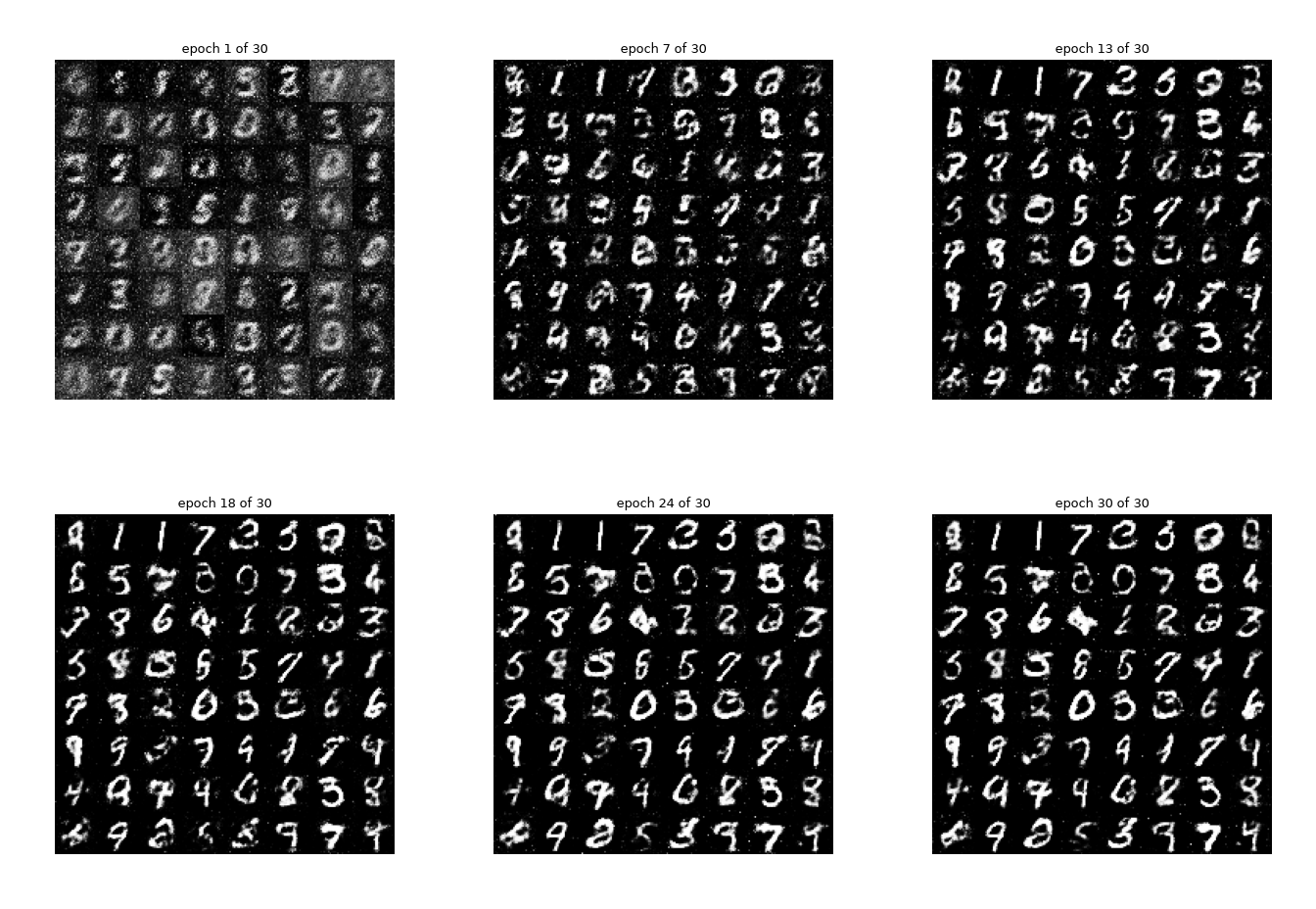The same 64 latent vectors, decoded after every epoch of training.

In [7]:

Copied!





# The final samples, larger
G.eval()
with torch.no_grad():
    final = G(torch.randn(64, LATENT_DIM, device=device)).cpu().numpy()

plt.figure(figsize=(7, 7))
plt.imshow(tile(final), cmap='gray', vmin=-1, vmax=1)
plt.axis('off')
plt.title('64 digits that do not exist')
plt.show()
# The final samples, larger
G.eval()
with torch.no_grad():
    final = G(torch.randn(64, LATENT_DIM, device=device)).cpu().numpy()

plt.figure(figsize=(7, 7))
plt.imshow(tile(final), cmap='gray', vmin=-1, vmax=1)
plt.axis('off')
plt.title('64 digits that do not exist')
plt.show()

6. Mode Collapse and Other Failures¶

GANs fail in characteristic ways, and knowing the symptoms saves hours.

Mode collapse is the notorious one. The generator discovers one output that reliably fools the discriminator and produces variations of only that — perfect 3s, and nothing else. It is a rational response to the objective: nothing in the loss rewards diversity, only plausibility.

You can detect it without labels by measuring how different the samples are from each other. Real MNIST digits vary a lot; a collapsed generator's samples do not.

In [8]:

Copied!





def diversity_score(images):
    """Mean pairwise distance between samples - a rough proxy for variety."""
    flat = images.reshape(len(images), -1)
    flat = torch.tensor(flat, dtype=torch.float32)
    dists = torch.cdist(flat, flat)
    n = len(flat)
    return dists.sum().item() / (n * (n - 1))      # exclude the zero diagonal

real_batch = next(iter(train_loader))[0].numpy()
print(f'Real images         : {diversity_score(real_batch[:64]):.3f}')
print(f'Generated (epoch 1) : {diversity_score(snapshots[0]):.3f}')
print(f'Generated (final)   : {diversity_score(snapshots[-1]):.3f}')
print('\nIf the generated score sits far below the real one, the generator has collapsed')
print('onto a few modes. Rising towards the real score means it is covering the data.')

plt.figure(figsize=(7, 4))
plt.plot([diversity_score(s) for s in snapshots], label='generated')
plt.axhline(diversity_score(real_batch[:64]), color='gray', linestyle='--', label='real data')
plt.xlabel('Epoch'); plt.ylabel('Mean pairwise distance')
plt.title('Sample diversity over training')
plt.legend(); plt.grid(alpha=0.3)
plt.show()
def diversity_score(images):
    """Mean pairwise distance between samples - a rough proxy for variety."""
    flat = images.reshape(len(images), -1)
    flat = torch.tensor(flat, dtype=torch.float32)
    dists = torch.cdist(flat, flat)
    n = len(flat)
    return dists.sum().item() / (n * (n - 1))      # exclude the zero diagonal

real_batch = next(iter(train_loader))[0].numpy()
print(f'Real images         : {diversity_score(real_batch[:64]):.3f}')
print(f'Generated (epoch 1) : {diversity_score(snapshots[0]):.3f}')
print(f'Generated (final)   : {diversity_score(snapshots[-1]):.3f}')
print('\nIf the generated score sits far below the real one, the generator has collapsed')
print('onto a few modes. Rising towards the real score means it is covering the data.')

plt.figure(figsize=(7, 4))
plt.plot([diversity_score(s) for s in snapshots], label='generated')
plt.axhline(diversity_score(real_batch[:64]), color='gray', linestyle='--', label='real data')
plt.xlabel('Epoch'); plt.ylabel('Mean pairwise distance')
plt.title('Sample diversity over training')
plt.legend(); plt.grid(alpha=0.3)
plt.show()

Real images         : 20.303
Generated (epoch 1) : 13.332
Generated (final)   : 19.813

If the generated score sits far below the real one, the generator has collapsed
onto a few modes. Rising towards the real score means it is covering the data.

The other failure modes:

Symptom	What is happening	What to try
`D(fake)` collapses to 0, G loss climbs	The discriminator won; G gets no gradient	Weaken D (dropout, fewer parameters, lower lr), label smoothing
`D(real)` and `D(fake)` both stuck at 0.5 with poor samples	D is too weak to teach anything	Strengthen D, or train it more often per G step
Samples oscillate between styles forever	Non-convergence; the two are chasing each other	Lower learning rates, use `betas=(0.5, 0.999)`, try WGAN-GP
All samples nearly identical	Mode collapse	Minibatch discrimination, unrolled GANs, WGAN-GP
Checkerboard artefacts in conv GANs	`ConvTranspose2d` stride overlap	Use upsample + conv, or kernel sizes divisible by the stride

The standard stabilisers, most from the DCGAN paper and the community lore that followed:

Normalise inputs to $[-1, 1]$ and end the generator with tanh.
LeakyReLU in the discriminator; avoid dead units.
BatchNorm in the generator, but not in the discriminator's first layer.
Adam with lr=2e-4, betas=(0.5, 0.999).
One-sided label smoothing on the real labels.
In convolutional GANs, use strided convolutions instead of pooling.

7. The Latent Space Is Structured Too¶

Like the VAE's, the generator's input space turns out to be smooth: walking a straight line between two latent vectors produces a continuous morph rather than a cut. Nothing in the loss asked for this — it falls out of training a continuous function.

In [9]:

Copied!





G.eval()
with torch.no_grad():
    z1 = torch.randn(1, LATENT_DIM, device=device)
    z2 = torch.randn(1, LATENT_DIM, device=device)
    steps = 50
    alphas = torch.linspace(0, 1, steps, device=device).view(-1, 1)
    z_path = (1 - alphas) * z1 + alphas * z2
    morph = G(z_path).cpu().numpy()

# a static strip ...
fig, axes = plt.subplots(1, 10, figsize=(12, 1.5))
for ax, img in zip(axes, morph[::5]):
    ax.imshow(img[0], cmap='gray', vmin=-1, vmax=1); ax.axis('off')
fig.suptitle('Interpolating between two random latent vectors', fontsize=10)
plt.tight_layout()
plt.show()
G.eval()
with torch.no_grad():
    z1 = torch.randn(1, LATENT_DIM, device=device)
    z2 = torch.randn(1, LATENT_DIM, device=device)
    steps = 50
    alphas = torch.linspace(0, 1, steps, device=device).view(-1, 1)
    z_path = (1 - alphas) * z1 + alphas * z2
    morph = G(z_path).cpu().numpy()

# a static strip ...
fig, axes = plt.subplots(1, 10, figsize=(12, 1.5))
for ax, img in zip(axes, morph[::5]):
    ax.imshow(img[0], cmap='gray', vmin=-1, vmax=1); ax.axis('off')
fig.suptitle('Interpolating between two random latent vectors', fontsize=10)
plt.tight_layout()
plt.show()

In [10]:

Copied!





# ... and the same walk as an animation
fig, ax = plt.subplots(figsize=(3.2, 3.4))
im = ax.imshow(morph[0][0], cmap='gray', vmin=-1, vmax=1)
ax.axis('off')

def update(k):
    im.set_data(morph[k][0])
    ax.set_title(f'step {k + 1} / {steps}', fontsize=10)
    return [im]

ani = animation.FuncAnimation(fig, update, frames=steps, interval=90, blit=False)
plt.close(fig)
save_animation(ani, 'lab16_morph.gif', fps=11)
# ... and the same walk as an animation
fig, ax = plt.subplots(figsize=(3.2, 3.4))
im = ax.imshow(morph[0][0], cmap='gray', vmin=-1, vmax=1)
ax.axis('off')

def update(k):
    im.set_data(morph[k][0])
    ax.set_title(f'step {k + 1} / {steps}', fontsize=10)
    return [im]

ani = animation.FuncAnimation(fig, update, frames=steps, interval=90, blit=False)
plt.close(fig)
save_animation(ani, 'lab16_morph.gif', fps=11)

saved Misc\lab16_morph.gif  (0.2 MB)

Out[10]:

'Misc\\lab16_morph.gif'

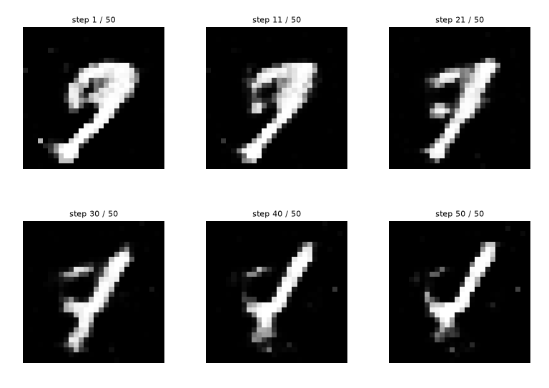Interpolating between two random latent vectors.

8. Experiment: Try Different Architectures and Hyperparameters¶

You can experiment with:

Building a DCGAN: replace the MLPs with nn.ConvTranspose2d in the generator and strided nn.Conv2d in the discriminator. Sharper digits, more compute.
Training the discriminator twice per generator step (or the reverse) and watching the balance shift
Removing the label smoothing, or the betas=(0.5, 0.999), to see how much they were doing
Making the discriminator much larger than the generator, to provoke the "D wins" failure on purpose
Implementing a conditional GAN: concatenate a one-hot digit label to both $z$ and the discriminator input, and you can then ask for a specific digit
Switching to the WGAN-GP objective, which replaces the BCE with an Earth-Mover distance plus a gradient penalty and is far more stable
Training on FashionMNIST and looking for mode collapse — it is easier to provoke there

Try modifying the model definition or training loop above and observe how the performance changes.

9. Conclusion¶

In this lab, you trained two networks against each other. The generator never saw a real image; everything it learned came through the discriminator's gradient. That is a genuinely different way to specify a learning problem — instead of writing down what "good" means, you train a second model to decide.

Key takeaways:

The generator's loss function is another neural network, and it keeps changing.
Use the non-saturating generator loss, or early training stalls.
.detach() the fakes in the discriminator step, or you will train the generator backwards.
Loss curves are not a progress bar here: watch D(real) and D(fake) converge on 0.5, and look at the samples.
Mode collapse is the characteristic failure, and nothing in the objective prevents it.
The architecture and optimizer details in the DCGAN recipe are not superstition — they carry real stability.

GANs, VAEs and diffusion models are three answers to the same question. VAEs optimise a bound on the likelihood and give you a clean latent space; GANs optimise against a learned critic and give you sharpness; diffusion models learn to reverse a noising process and currently give the best of both.

The next and final lab is about everything that comes after training: getting a model out of the notebook and into something that runs.