Lab 15: Autoencoders and Variational Autoencoders
Every model so far needed labels. This lab does not. Autoencoders learn by trying to reproduce their own input, which means any pile of unlabelled data is a training set — and that is most data.
Then we make one change to the architecture, and the model stops merely compressing data and starts generating it.
We will cover the following topics:
- Autoencoders: compression as a learning signal
- Reading the latent space, and what it is good for
- Denoising autoencoders
- Why a plain autoencoder cannot generate, and what breaks
- Variational autoencoders: the reparameterization trick and the ELBO
- Sampling and interpolating in a learned latent space
1. Learning Without Labels
An autoencoder is two networks trained as one:
- an encoder that squeezes the input $x$ into a small vector $z$
- a decoder that tries to rebuild $x$ from $z$ alone
The loss is simply how far the output is from the input. No labels anywhere.

The bottleneck is what makes this non-trivial. If $z$ were as large as $x$, the network could learn the identity function and learn nothing. Forcing $z$ to be much smaller means the encoder has to decide what is worth keeping — and "what is worth keeping" is exactly what we mean by a useful representation.
Autoencoders are used for dimensionality reduction, denoising, anomaly detection (things the model reconstructs badly are unusual), and pretraining.
import torch
import torch.nn as nn
import torch.optim as optim
import numpy as np
import matplotlib.pyplot as plt
from torch.utils.data import DataLoader
from torchvision import datasets, transforms

torch.manual_seed(0)
np.random.seed(0)
device = torch.device('cuda' if torch.cuda.is_available() else 'cpu')
print('PyTorch version:', torch.__version__, '| device:', device)

# No normalisation here: we want pixels in [0, 1] so the decoder can end in a sigmoid
tf = transforms.ToTensor()
train_set = datasets.MNIST(root='./data', train=True, download=True, transform=tf)
test_set = datasets.MNIST(root='./data', train=False, download=True, transform=tf)

train_loader = DataLoader(train_set, batch_size=256, shuffle=True)
test_loader = DataLoader(test_set, batch_size=512, shuffle=False)
print(f'{len(train_set)} training images, {len(test_set)} test images, no labels used')
PyTorch version: 2.13.0+cpu | device: cpu
60000 training images, 10000 test images, no labels used
2. Building an Autoencoder
A symmetric pair of MLPs. The only design decision that really matters is the size of the bottleneck.
The decoder ends in a sigmoid because our pixels live in $[0, 1]$, and the loss is binary cross-entropy — the standard choice for MNIST, which treats each pixel as an independent probability of being "on". Mean squared error also works and gives blurrier results.
class Autoencoder(nn.Module):
    def __init__(self, latent_dim=32):
        super(Autoencoder, self).__init__()
        self.latent_dim = latent_dim
        self.encoder = nn.Sequential(
            nn.Linear(784, 256), nn.ReLU(),
            nn.Linear(256, 64), nn.ReLU(),
            nn.Linear(64, latent_dim),
        )
        self.decoder = nn.Sequential(
            nn.Linear(latent_dim, 64), nn.ReLU(),
            nn.Linear(64, 256), nn.ReLU(),
            nn.Linear(256, 784), nn.Sigmoid(),
        )

    def forward(self, x):
        flat = x.view(x.size(0), -1)
        z = self.encoder(flat)
        out = self.decoder(z)
        return out.view_as(x), z

model = Autoencoder(latent_dim=32)
print(model)
print(f'\nCompression: 784 pixels -> {model.latent_dim} numbers '
      f'({784 / model.latent_dim:.0f}x)')
Autoencoder(
  (encoder): Sequential(
    (0): Linear(in_features=784, out_features=256, bias=True)
    (1): ReLU()
    (2): Linear(in_features=256, out_features=64, bias=True)
    (3): ReLU()
    (4): Linear(in_features=64, out_features=32, bias=True)
  )
  (decoder): Sequential(
    (0): Linear(in_features=32, out_features=64, bias=True)
    (1): ReLU()
    (2): Linear(in_features=64, out_features=256, bias=True)
    (3): ReLU()
    (4): Linear(in_features=256, out_features=784, bias=True)
    (5): Sigmoid()
  )
)

Compression: 784 pixels -> 32 numbers (24x)
def train_autoencoder(model, epochs=8, lr=1e-3, label=''):
    model = model.to(device)
    optimizer = optim.Adam(model.parameters(), lr=lr)
    criterion = nn.BCELoss(reduction='sum')       # summed over pixels, averaged over batch
    history = []

    for epoch in range(epochs):
        model.train()
        running = 0.0
        for images, _ in train_loader:            # labels deliberately ignored
            images = images.to(device)
            recon, _ = model(images)
            loss = criterion(recon, images) / images.size(0)
            optimizer.zero_grad()
            loss.backward()
            optimizer.step()
            running += loss.item() * images.size(0)
        history.append(running / len(train_set))
        print(f'  [{label}] epoch {epoch+1}/{epochs}  loss {history[-1]:.2f}')
    return history

print('Training the autoencoder (latent_dim = 32):')
ae_history = train_autoencoder(model, epochs=8, label='ae32')
Training the autoencoder (latent_dim = 32):
[ae32] epoch 1/8 loss 207.67
[ae32] epoch 2/8 loss 133.79
[ae32] epoch 3/8 loss 113.40
[ae32] epoch 4/8 loss 104.86
[ae32] epoch 5/8 loss 99.21
[ae32] epoch 6/8 loss 94.54
[ae32] epoch 7/8 loss 90.84
[ae32] epoch 8/8 loss 88.33
def show_reconstructions(model, n=8, title=''):
    model.eval()
    images, labels = next(iter(test_loader))
    with torch.no_grad():
        recon, _ = model(images[:n].to(device))
    recon = recon.cpu()

    fig, axes = plt.subplots(2, n, figsize=(1.3 * n, 3))
    for i in range(n):
        axes[0, i].imshow(images[i][0], cmap='gray'); axes[0, i].axis('off')
        axes[1, i].imshow(recon[i][0], cmap='gray'); axes[1, i].axis('off')
    axes[0, 0].set_title('original', loc='left', fontsize=9)
    axes[1, 0].set_title('reconstructed', loc='left', fontsize=9)
    fig.suptitle(title)
    plt.tight_layout()
    plt.show()

show_reconstructions(model, title='Autoencoder with a 32-dimensional bottleneck')

How narrow can the bottleneck get?
The bottleneck size is a direct dial between compression and fidelity. Let's train the same architecture at several latent sizes and look at what survives.
latent_sizes = [2, 8, 32]
ae_models = {}
for d in latent_sizes:
    torch.manual_seed(0)
    print(f'latent_dim = {d}')
    m = Autoencoder(latent_dim=d)
    train_autoencoder(m, epochs=6, label=f'ae{d}')
    ae_models[d] = m
latent_dim = 2
[ae2] epoch 1/6 loss 210.91
[ae2] epoch 2/6 loss 170.16
[ae2] epoch 3/6 loss 160.63
[ae2] epoch 4/6 loss 154.97
[ae2] epoch 5/6 loss 151.22
  [ae2] epoch 6/6  loss 148.67
latent_dim = 8
[ae8] epoch 1/6 loss 207.91
[ae8] epoch 2/6 loss 137.45
[ae8] epoch 3/6 loss 118.55
[ae8] epoch 4/6 loss 112.29
[ae8] epoch 5/6 loss 107.52
  [ae8] epoch 6/6  loss 104.82
latent_dim = 32
[ae32] epoch 1/6 loss 207.67
[ae32] epoch 2/6 loss 133.79
[ae32] epoch 3/6 loss 113.40
[ae32] epoch 4/6 loss 104.86
[ae32] epoch 5/6 loss 99.21
[ae32] epoch 6/6 loss 94.54
images, labels = next(iter(test_loader))
n = 8
fig, axes = plt.subplots(len(latent_sizes) + 1, n, figsize=(1.3 * n, 1.5 * (len(latent_sizes) + 1)))
for i in range(n):
    axes[0, i].imshow(images[i][0], cmap='gray'); axes[0, i].axis('off')
axes[0, 0].set_ylabel('original')
axes[0, 0].set_title('original', loc='left', fontsize=9)

for row, d in enumerate(latent_sizes, start=1):
    ae_models[d].eval()
    with torch.no_grad():
        recon, _ = ae_models[d](images[:n].to(device))
    for i in range(n):
        axes[row, i].imshow(recon[i][0].cpu(), cmap='gray'); axes[row, i].axis('off')
    axes[row, 0].set_title(f'latent_dim = {d}', loc='left', fontsize=9)
plt.tight_layout()
plt.show()
print('At 2 dimensions the network can only keep the broadest shape - the identity of the')
print('digit is often lost. That is 784 numbers squeezed into 2.')

At 2 dimensions the network can only keep the broadest shape - the identity of the
digit is often lost. That is 784 numbers squeezed into 2.
3. Reading the Latent Space
A 2-dimensional bottleneck is bad for reconstruction but perfect for looking at. We can plot every test digit at its latent coordinates and colour by the true label — labels the model never saw.
If similar digits land near each other, the encoder has discovered structure on its own.
def encode_dataset(model, loader, limit=5000):
    model.eval()
    zs, ys = [], []
    with torch.no_grad():
        for images, labels in loader:
            _, z = model(images.to(device))
            zs.append(z.cpu())
            ys.append(labels)
            if sum(len(a) for a in zs) >= limit:
                break
    return torch.cat(zs)[:limit].numpy(), torch.cat(ys)[:limit].numpy()

z2, y2 = encode_dataset(ae_models[2], test_loader)

plt.figure(figsize=(6.5, 5.5))
scatter = plt.scatter(z2[:, 0], z2[:, 1], c=y2, cmap='tab10', s=6, alpha=0.7)
plt.colorbar(scatter, label='true digit (never shown to the model)')
plt.xlabel('$z_1$'); plt.ylabel('$z_2$')
plt.title('The 2-D latent space of a plain autoencoder')
plt.grid(alpha=0.2)
plt.show()

The digits do separate into clusters — genuine unsupervised structure. But look at the geometry: the clusters have irregular shapes, wildly different scales, and large empty regions between them. That will matter in a moment.
4. Denoising Autoencoders
A useful variant: corrupt the input, but ask for the clean image back. The network cannot copy any more — it has to understand what a digit looks like well enough to repair one.
The only change is in the training loop: noisy in, clean out.
def train_denoising(model, epochs=8, noise=0.4, lr=1e-3, label='dae'):
    model = model.to(device)
    optimizer = optim.Adam(model.parameters(), lr=lr)
    criterion = nn.BCELoss(reduction='sum')
    history = []

    for epoch in range(epochs):
        model.train()
        running = 0.0
        for images, _ in train_loader:
            images = images.to(device)
            noisy = (images + noise * torch.randn_like(images)).clamp(0, 1)
            recon, _ = model(noisy)               # corrupted input ...
            loss = criterion(recon, images) / images.size(0)   # ... clean target
            optimizer.zero_grad()
            loss.backward()
            optimizer.step()
            running += loss.item() * images.size(0)
        history.append(running / len(train_set))
        print(f'  [{label}] epoch {epoch+1}/{epochs}  loss {history[-1]:.2f}')
    return history

torch.manual_seed(0)
denoiser = Autoencoder(latent_dim=32)
train_denoising(denoiser, epochs=8)
[dae] epoch 1/8 loss 218.77
[dae] epoch 2/8 loss 165.91
[dae] epoch 3/8 loss 129.05
[dae] epoch 4/8 loss 118.97
[dae] epoch 5/8 loss 112.53
[dae] epoch 6/8 loss 108.26
[dae] epoch 7/8 loss 105.24
[dae] epoch 8/8 loss 103.02
[218.76724349772135,
 165.9106280110677,
 129.04570998128256,
 118.97151585286458,
 112.52704283447265,
 108.2648680053711,
 105.23613069661458,
 103.02289713134766]
denoiser.eval()
images, _ = next(iter(test_loader))
clean = images[:8].to(device)
noisy = (clean + 0.4 * torch.randn_like(clean)).clamp(0, 1)
with torch.no_grad():
    repaired, _ = denoiser(noisy)

fig, axes = plt.subplots(3, 8, figsize=(10, 4))
for i in range(8):
    axes[0, i].imshow(clean[i][0].cpu(), cmap='gray'); axes[0, i].axis('off')
    axes[1, i].imshow(noisy[i][0].cpu(), cmap='gray'); axes[1, i].axis('off')
    axes[2, i].imshow(repaired[i][0].cpu(), cmap='gray'); axes[2, i].axis('off')
for ax, name in zip(axes[:, 0], ['clean', 'noisy input', 'repaired']):
    ax.set_title(name, loc='left', fontsize=9)
plt.tight_layout()
plt.show()

5. Why an Autoencoder Cannot Generate
Here is a tempting idea: the decoder maps latent vectors to images, so why not feed it a random vector and get a new digit?
Try it. The result is the reason variational autoencoders exist.
ae2 = ae_models[2]
ae2.eval()

# Sample from the region the encoder actually uses
z_min, z_max = z2.min(axis=0), z2.max(axis=0)
random_z = torch.tensor(
    np.random.uniform(z_min, z_max, size=(8, 2)), dtype=torch.float32, device=device)

with torch.no_grad():
    generated = ae2.decoder(random_z).view(-1, 28, 28).cpu()

fig, axes = plt.subplots(1, 8, figsize=(10, 1.6))
for ax, img in zip(axes, generated):
    ax.imshow(img, cmap='gray'); ax.axis('off')
fig.suptitle('Decoding random points from a plain autoencoder', fontsize=10)
plt.tight_layout()
plt.show()

Mostly smudges. The problem is structural, not a matter of training longer:
- The latent space has holes. The encoder was never asked to use the space between clusters, so the decoder was never trained there and produces nonsense.
- We do not know the distribution of $z$. To sample properly you need to know where the valid codes live, and a plain autoencoder never tells you.
- It is not continuous. Nearby codes need not decode to similar images, so interpolation passes through garbage.
A VAE fixes all three by making the encoder output a distribution instead of a point, and penalising it for drifting away from a standard normal.
6. The Variational Autoencoder
The VAE changes the encoder to emit two vectors — a mean $\mu$ and a log-variance $\log \sigma^2$ — which together define a Gaussian. We sample $z$ from that Gaussian and decode it.
The loss has two terms:
$$ \mathcal{L} = \underbrace{\mathbb{E}_{q(z|x)}\left[-\log p(x|z)\right]}_{\text{reconstruction}} \; + \; \underbrace{D_{KL}\!\left(q(z|x)\,\|\,\mathcal{N}(0, I)\right)}_{\text{regularization}} $$
The first term is the familiar reconstruction loss. The second is a KL divergence pulling every encoded Gaussian towards the standard normal, which is what fills the holes: overlapping, unit-scale Gaussians tile the space with no gaps. For diagonal Gaussians it has a closed form:
$$ D_{KL} = -\frac{1}{2} \sum_{j} \left(1 + \log \sigma_j^2 - \mu_j^2 - \sigma_j^2\right) $$
The two terms pull against each other. Reconstruction wants precise, well-separated codes; the KL term wants every input mapped to the same standard normal. The balance is what produces a latent space that is both informative and continuous.
The reparameterization trick
There is one obstacle: sampling is not differentiable. You cannot backpropagate through "draw a random number", so gradients would never reach the encoder.
The fix is to move the randomness out of the path. Instead of sampling $z \sim \mathcal{N}(\mu, \sigma^2)$ directly, sample a parameter-free $\epsilon \sim \mathcal{N}(0, I)$ and compute
$$ z = \mu + \sigma \odot \epsilon $$
which has exactly the same distribution — but now $z$ is a deterministic function of $\mu$ and $\sigma$, with the randomness supplied as an input. Gradients flow straight through.

class VAE(nn.Module):
    def __init__(self, latent_dim=2):
        super(VAE, self).__init__()
        self.latent_dim = latent_dim
        self.encoder = nn.Sequential(
            nn.Linear(784, 256), nn.ReLU(),
            nn.Linear(256, 64), nn.ReLU(),
        )
        self.fc_mu = nn.Linear(64, latent_dim)          # the mean
        self.fc_logvar = nn.Linear(64, latent_dim)      # the log-variance
        self.decoder = nn.Sequential(
            nn.Linear(latent_dim, 64), nn.ReLU(),
            nn.Linear(64, 256), nn.ReLU(),
            nn.Linear(256, 784), nn.Sigmoid(),
        )

    def encode(self, x):
        h = self.encoder(x.view(x.size(0), -1))
        return self.fc_mu(h), self.fc_logvar(h)

    def reparameterize(self, mu, logvar):
        std = torch.exp(0.5 * logvar)         # we predict log-variance for stability
        eps = torch.randn_like(std)           # the randomness, with no parameters
        return mu + std * eps                 # differentiable in mu and std

    def forward(self, x):
        mu, logvar = self.encode(x)
        z = self.reparameterize(mu, logvar)
        recon = self.decoder(z).view_as(x)
        return recon, mu, logvar, z

def vae_loss(recon, x, mu, logvar, beta=1.0):
    """Reconstruction + beta * KL, summed over dimensions and averaged over the batch."""
    recon_loss = nn.functional.binary_cross_entropy(recon, x, reduction='sum')
    kl = -0.5 * torch.sum(1 + logvar - mu.pow(2) - logvar.exp())
    return (recon_loss + beta * kl) / x.size(0), recon_loss / x.size(0), kl / x.size(0)
Why predict $\log \sigma^2$ rather than $\sigma$? A variance must be positive, and a raw linear layer can output anything. Exponentiating a log-variance guarantees positivity, and it keeps the numbers on a well-behaved scale — the same reason we use logits instead of probabilities everywhere else.
def train_vae(model, epochs=12, lr=1e-3, beta=1.0, label='vae'):
    model = model.to(device)
    optimizer = optim.Adam(model.parameters(), lr=lr)
    history = {'total': [], 'recon': [], 'kl': []}

    for epoch in range(epochs):
        model.train()
        totals = np.zeros(3)
        for images, _ in train_loader:
            images = images.to(device)
            recon, mu, logvar, _ = model(images)
            loss, rec, kl = vae_loss(recon, images, mu, logvar, beta)
            optimizer.zero_grad()
            loss.backward()
            optimizer.step()
            totals += np.array([loss.item(), rec.item(), kl.item()]) * images.size(0)
        totals /= len(train_set)
        for key, value in zip(['total', 'recon', 'kl'], totals):
            history[key].append(value)
        print(f'  [{label}] epoch {epoch+1}/{epochs}  '
              f'total {totals[0]:.2f}  recon {totals[1]:.2f}  KL {totals[2]:.2f}')
    return history

torch.manual_seed(0)
vae = VAE(latent_dim=2)
vae_history = train_vae(vae, epochs=12)

plt.figure(figsize=(7, 4))
plt.plot(vae_history['recon'], label='reconstruction term')
plt.plot(vae_history['kl'], label='KL term')
plt.plot(vae_history['total'], label='total', linestyle='--')
plt.xlabel('Epoch'); plt.ylabel('Loss per image')
plt.title('The two terms of the VAE objective')
plt.legend(); plt.grid(alpha=0.3)
plt.show()
[vae] epoch 1/12 total 212.30 recon 208.84 KL 3.46
[vae] epoch 2/12 total 172.28 recon 167.61 KL 4.67
[vae] epoch 3/12 total 164.62 recon 159.52 KL 5.11
[vae] epoch 4/12 total 161.53 recon 156.26 KL 5.27
[vae] epoch 5/12 total 159.15 recon 153.75 KL 5.40
[vae] epoch 6/12 total 157.31 recon 151.82 KL 5.48
[vae] epoch 7/12 total 155.93 recon 150.35 KL 5.58
[vae] epoch 8/12 total 154.61 recon 148.96 KL 5.65
[vae] epoch 9/12 total 153.39 recon 147.68 KL 5.70
[vae] epoch 10/12 total 152.26 recon 146.48 KL 5.78
[vae] epoch 11/12 total 151.25 recon 145.42 KL 5.83
[vae] epoch 12/12 total 150.45 recon 144.57 KL 5.88

7. A Latent Space You Can Sample From
Now compare the two latent spaces side by side. The VAE's should be centred on the origin, roughly unit-scale, and gap-free — because that is precisely what the KL term asked for.
vae.eval()
mus, ys = [], []
with torch.no_grad():
    for images, labels in test_loader:
        mu, _ = vae.encode(images.to(device))
        mus.append(mu.cpu()); ys.append(labels)
        if sum(len(m) for m in mus) >= 5000:
            break
zv = torch.cat(mus)[:5000].numpy()
yv = torch.cat(ys)[:5000].numpy()

fig, (ax1, ax2) = plt.subplots(1, 2, figsize=(12, 5))
for ax, z, y, title in [(ax1, z2, y2, 'plain autoencoder'),
                        (ax2, zv, yv, 'variational autoencoder')]:
    s = ax.scatter(z[:, 0], z[:, 1], c=y, cmap='tab10', s=6, alpha=0.7)
    ax.set_title(title)
    ax.set_xlabel('$z_1$'); ax.set_ylabel('$z_2$')
    ax.grid(alpha=0.2)
fig.colorbar(s, ax=[ax1, ax2], label='true digit', fraction=0.02)
plt.show()

print('Plain AE  latent range:', z2.min(axis=0).round(2), 'to', z2.max(axis=0).round(2))
print('VAE       latent range:', zv.min(axis=0).round(2), 'to', zv.max(axis=0).round(2))
print('The VAE\'s codes sit where the prior N(0, I) says they should - so we can sample there.')

Plain AE  latent range: [-21.24 -22.58] to [8.98 9.41]
VAE       latent range: [-3.48 -3.79] to [3.18 3.43]
The VAE's codes sit where the prior N(0, I) says they should - so we can sample there.
# Generate digits that do not exist: sample straight from the prior
with torch.no_grad():
    z_prior = torch.randn(16, vae.latent_dim, device=device)
    samples = vae.decoder(z_prior).view(-1, 28, 28).cpu()

fig, axes = plt.subplots(2, 8, figsize=(10, 2.8))
for ax, img in zip(axes.ravel(), samples):
    ax.imshow(img, cmap='gray'); ax.axis('off')
fig.suptitle('Sampled from $z \\sim \\mathcal{N}(0, I)$ - no input image involved')
plt.tight_layout()
plt.show()

The learned manifold
With a 2-D latent space we can decode a whole grid of codes and see the entire space the model learned at once. Digits should morph smoothly into their neighbours, with no dead regions — the property the plain autoencoder lacked.
from scipy.stats import norm

grid_n = 18
# Walk the prior by quantile, so the grid covers the region the model actually uses
coords = norm.ppf(np.linspace(0.02, 0.98, grid_n))
canvas = np.zeros((grid_n * 28, grid_n * 28))

vae.eval()
with torch.no_grad():
    for i, yi in enumerate(coords[::-1]):
        row = torch.tensor([[xi, yi] for xi in coords], dtype=torch.float32, device=device)
        decoded = vae.decoder(row).view(-1, 28, 28).cpu().numpy()
        for j, img in enumerate(decoded):
            canvas[i * 28:(i + 1) * 28, j * 28:(j + 1) * 28] = img

plt.figure(figsize=(8, 8))
plt.imshow(canvas, cmap='gray')
plt.xticks([]); plt.yticks([])
plt.title('The learned 2-D manifold, decoded on a grid')
plt.show()

Walking through latent space
Interpolating between two encoded digits shows the same thing in motion. Because the space is continuous, every intermediate point decodes to something plausible — the digit becomes another digit rather than dissolving.
from matplotlib import animation
import os

os.makedirs('Misc', exist_ok=True)

def save_animation(ani, filename, fps=8, dpi=80):
    """Render an animation to a GIF under Misc/ and report where it went."""
    path = os.path.join('Misc', filename)
    ani.save(path, writer='pillow', fps=fps, dpi=dpi)
    print(f'saved {path}  ({os.path.getsize(path) / 1e6:.1f} MB)')
    return path

# Pick two test images with different labels and walk between their codes
images, labels = next(iter(test_loader))
idx_a = 0
idx_b = int(np.where(labels.numpy() != labels[0].item())[0][0])

vae.eval()
with torch.no_grad():
    mu_a, _ = vae.encode(images[idx_a:idx_a + 1].to(device))
    mu_b, _ = vae.encode(images[idx_b:idx_b + 1].to(device))
    steps = 60
    alphas = torch.linspace(0, 1, steps, device=device).view(-1, 1)
    z_path = (1 - alphas) * mu_a + alphas * mu_b        # straight line in latent space
    frames = vae.decoder(z_path).view(-1, 28, 28).cpu().numpy()

fig, (ax_path, ax_img) = plt.subplots(1, 2, figsize=(9, 4))
ax_path.scatter(zv[:, 0], zv[:, 1], c=yv, cmap='tab10', s=4, alpha=0.35)
zp = z_path.cpu().numpy()
ax_path.plot(zp[:, 0], zp[:, 1], color='k', lw=1.2)
dot, = ax_path.plot([], [], 'o', color='red', markersize=9)
ax_path.set_xlabel('$z_1$'); ax_path.set_ylabel('$z_2$')
ax_path.set_title('position in latent space')

im = ax_img.imshow(frames[0], cmap='gray', vmin=0, vmax=1)
ax_img.axis('off')
ax_img.set_title('decoded image')

def update(k):
    dot.set_data([zp[k, 0]], [zp[k, 1]])
    im.set_data(frames[k])
    return dot, im

ani = animation.FuncAnimation(fig, update, frames=steps, interval=80, blit=False)
plt.close(fig)
save_animation(ani, 'lab15_latent_walk.gif', fps=12)
saved Misc\lab15_latent_walk.gif (1.9 MB)
'Misc\\lab15_latent_walk.gif'
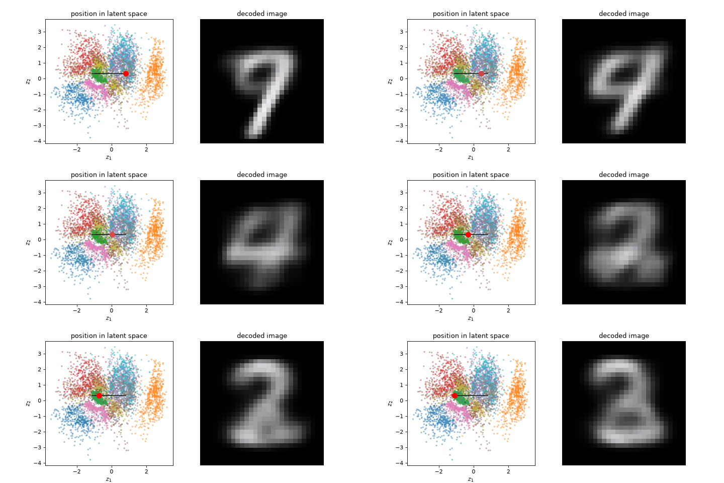 Walking a straight line through the VAE latent space, with no dead regions along the way.
8. Experiment: Try Different Architectures and Hyperparameters
You can experiment with:
- Changing
betainvae_loss:beta = 0reduces the VAE to a plain autoencoder, whilebeta = 4gives a "β-VAE" with a more disentangled but blurrier latent space - Training the VAE with
latent_dim = 16— sharper samples, but you lose the 2-D picture - Replacing the MLPs with convolutional encoders and
nn.ConvTranspose2ddecoders - Using MSE instead of BCE for the reconstruction term and comparing the sharpness
- Training a VAE on FashionMNIST and walking its manifold
- Building an anomaly detector: train on digits 0-8 only, then check whether 9s get a higher reconstruction error
- Interpolating between two points in the plain autoencoder's latent space, to see the difference the KL term made
Try modifying the model definition or training loop above and observe how the performance changes.
9. Conclusion
In this lab, you trained networks with no labels at all. An autoencoder learns by reconstructing its input through a bottleneck, which forces it to discover what matters. A variational autoencoder adds a probabilistic encoder and a KL penalty, turning that bottleneck into a smooth, samplable latent space — and a compression model into a generative one.
Key takeaways:
- The bottleneck is the teacher: without it there is nothing to learn.
- A plain autoencoder's latent space has holes, so you cannot sample from it.
- The reparameterization trick moves randomness into an input so gradients can pass through.
- The KL term shapes the latent space towards $\mathcal{N}(0, I)$; the reconstruction term fights it, and the balance is the model.
- Predict
logvar, notsigma, for positivity and numerical stability. - Denoising is a one-line change to the training loop and gives more robust features.
VAEs generate by reconstructing, which is why their samples look slightly blurry — averaging is the safest way to minimise reconstruction loss. The next lab takes the opposite approach: train a second network whose only job is to notice blur.