Lab 13: Regularization and Optimization¶

Up to now, every lab has focused on architecture — what the network is. This one is about everything else: the choices that decide whether the network you built actually learns, and whether what it learns generalises to data it has never seen.

These techniques matter more in practice than the choice of architecture. A well-regularized simple model beats a badly-trained sophisticated one almost every time.

We will cover the following topics:

• Diagnosing overfitting and underfitting from the loss curves
• The regularization toolkit: weight decay, dropout, batch normalization, augmentation, early stopping
• How optimizers actually move through the loss landscape
• Learning rate: the single most important hyperparameter, and how to schedule it
• Combining everything and measuring what each piece bought us

A note on runtime. This lab trains around eighteen models, so that every claim below is measured rather than asserted. Start to finish it takes roughly 25 minutes on a laptop CPU, most of it in sections 3 to 6 and section 10. If you want to explore quickly first, drop epochs from 40 to 15 in the fit calls — the shape of every result stays the same, only the final numbers shift.

1. The Problem: Generalization¶

Training a network is easy. Making it work on new data is the hard part.

• Underfitting: the model is too weak, or trained too briefly. Training loss stays high. Both curves are bad.
• Overfitting: the model memorises the training set instead of learning the pattern. Training loss keeps falling while validation loss turns around and climbs.

The gap between the two curves is the overfitting, and watching it is how you diagnose a training run:

Regularization is the collective name for anything that trades a little training accuracy for better validation accuracy. Every technique in this lab is a different way of making the network's job slightly harder on purpose.

2. Setting Up a Model That Overfits¶

To study overfitting we need to provoke it. The recipe is reliable: a network with plenty of capacity, and not much data.

We will use FashionMNIST — same shape as MNIST, considerably harder — with only 2,000 training images and a deliberately oversized network.

In [1]:

import torch
import torch.nn as nn
import torch.optim as optim
import numpy as np
import matplotlib.pyplot as plt
from torch.utils.data import DataLoader, Subset
from torchvision import datasets, transforms

torch.manual_seed(0)
np.random.seed(0)
device = torch.device('cuda' if torch.cuda.is_available() else 'cpu')
print('PyTorch version:', torch.__version__, '| device:', device)

import torch import torch.nn as nn import torch.optim as optim import numpy as np import matplotlib.pyplot as plt from torch.utils.data import DataLoader, Subset from torchvision import datasets, transforms torch.manual_seed(0) np.random.seed(0) device = torch.device('cuda' if torch.cuda.is_available() else 'cpu') print('PyTorch version:', torch.__version__, '| device:', device)

PyTorch version: 2.13.0+cpu | device: cpu

In [2]:

base_tf = transforms.Compose([
    transforms.ToTensor(),
    transforms.Normalize((0.2860,), (0.3530,)),   # FashionMNIST mean and std
])

full_train = datasets.FashionMNIST(root='./data', train=True, download=True, transform=base_tf)
full_test = datasets.FashionMNIST(root='./data', train=False, download=True, transform=base_tf)

N_TRAIN = 2000
small_train = Subset(full_train, range(N_TRAIN))
val_set = Subset(full_test, range(2000))

train_loader = DataLoader(small_train, batch_size=64, shuffle=True)
val_loader = DataLoader(val_set, batch_size=512, shuffle=False)

CLASSES = full_train.classes
print(f'{len(small_train)} training images, {len(val_set)} validation images')
print('Classes:', CLASSES)

base_tf = transforms.Compose([ transforms.ToTensor(), transforms.Normalize((0.2860,), (0.3530,)), # FashionMNIST mean and std ]) full_train = datasets.FashionMNIST(root='./data', train=True, download=True, transform=base_tf) full_test = datasets.FashionMNIST(root='./data', train=False, download=True, transform=base_tf) N_TRAIN = 2000 small_train = Subset(full_train, range(N_TRAIN)) val_set = Subset(full_test, range(2000)) train_loader = DataLoader(small_train, batch_size=64, shuffle=True) val_loader = DataLoader(val_set, batch_size=512, shuffle=False) CLASSES = full_train.classes print(f'{len(small_train)} training images, {len(val_set)} validation images') print('Classes:', CLASSES)

2000 training images, 2000 validation images
Classes: ['T-shirt/top', 'Trouser', 'Pullover', 'Dress', 'Coat', 'Sandal', 'Shirt', 'Sneaker', 'Bag', 'Ankle boot']

In [3]:

images, labels = next(iter(train_loader))
fig, axes = plt.subplots(1, 8, figsize=(11, 1.8))
for ax, img, lab in zip(axes, images, labels):
    ax.imshow(img[0], cmap='gray')
    ax.set_title(CLASSES[lab], fontsize=7)
    ax.axis('off')
plt.tight_layout()
plt.show()

images, labels = next(iter(train_loader)) fig, axes = plt.subplots(1, 8, figsize=(11, 1.8)) for ax, img, lab in zip(axes, images, labels): ax.imshow(img[0], cmap='gray') ax.set_title(CLASSES[lab], fontsize=7) ax.axis('off') plt.tight_layout() plt.show()

In [4]:

class MLP(nn.Module):
    """A deliberately oversized network, with optional dropout and batch norm."""
    def __init__(self, hidden=512, dropout=0.0, batchnorm=False):
        super(MLP, self).__init__()
        layers = []
        in_dim = 28 * 28
        for _ in range(3):
            layers.append(nn.Linear(in_dim, hidden))
            if batchnorm:
                layers.append(nn.BatchNorm1d(hidden))
            layers.append(nn.ReLU())
            if dropout > 0:
                layers.append(nn.Dropout(dropout))
            in_dim = hidden
        layers.append(nn.Linear(hidden, 10))
        self.net = nn.Sequential(*layers)

    def forward(self, x):
        return self.net(x.view(x.size(0), -1))

probe = MLP()
print(f'{sum(p.numel() for p in probe.parameters()):,} parameters '
      f'for {N_TRAIN} training images - about '
      f'{sum(p.numel() for p in probe.parameters()) // N_TRAIN} parameters per image.')

class MLP(nn.Module): """A deliberately oversized network, with optional dropout and batch norm.""" def __init__(self, hidden=512, dropout=0.0, batchnorm=False): super(MLP, self).__init__() layers = [] in_dim = 28 * 28 for _ in range(3): layers.append(nn.Linear(in_dim, hidden)) if batchnorm: layers.append(nn.BatchNorm1d(hidden)) layers.append(nn.ReLU()) if dropout > 0: layers.append(nn.Dropout(dropout)) in_dim = hidden layers.append(nn.Linear(hidden, 10)) self.net = nn.Sequential(*layers) def forward(self, x): return self.net(x.view(x.size(0), -1)) probe = MLP() print(f'{sum(p.numel() for p in probe.parameters()):,} parameters ' f'for {N_TRAIN} training images - about ' f'{sum(p.numel() for p in probe.parameters()) // N_TRAIN} parameters per image.')

932,362 parameters for 2000 training images - about 466 parameters per image.

That ratio is the whole problem in one number. The network has more than enough capacity to store the training set outright, so unless we stop it, that is exactly what it will do.

In [5]:

criterion = nn.CrossEntropyLoss()

def run_epoch(model, loader, optimizer=None, clip=None):
    """One pass over a loader. Pass an optimizer to train, omit it to evaluate."""
    training = optimizer is not None
    model.train() if training else model.eval()
    total_loss = correct = total = 0

    with torch.set_grad_enabled(training):
        for images, labels in loader:
            images, labels = images.to(device), labels.to(device)
            outputs = model(images)
            loss = criterion(outputs, labels)
            if training:
                optimizer.zero_grad()
                loss.backward()
                if clip is not None:
                    nn.utils.clip_grad_norm_(model.parameters(), clip)
                optimizer.step()
            total_loss += loss.item() * images.size(0)
            correct += (outputs.argmax(1) == labels).sum().item()
            total += labels.size(0)
    return total_loss / total, 100 * correct / total

def fit(model, epochs=40, lr=1e-3, weight_decay=0.0, scheduler_fn=None,
        clip=None, verbose_every=10, label='', loader=None):
    loader = loader if loader is not None else train_loader
    model = model.to(device)
    optimizer = optim.Adam(model.parameters(), lr=lr, weight_decay=weight_decay)
    scheduler = scheduler_fn(optimizer) if scheduler_fn else None
    hist = {'train_loss': [], 'val_loss': [], 'train_acc': [], 'val_acc': [], 'lr': []}

    for epoch in range(epochs):
        tr_loss, tr_acc = run_epoch(model, loader, optimizer, clip)
        va_loss, va_acc = run_epoch(model, val_loader)
        hist['lr'].append(optimizer.param_groups[0]['lr'])
        if scheduler:
            scheduler.step()
        for key, value in zip(['train_loss', 'val_loss', 'train_acc', 'val_acc'],
                              [tr_loss, va_loss, tr_acc, va_acc]):
            hist[key].append(value)
        if verbose_every and (epoch + 1) % verbose_every == 0:
            print(f'  [{label}] epoch {epoch+1:3d}  train {tr_loss:.4f}/{tr_acc:5.1f}%  '
                  f'val {va_loss:.4f}/{va_acc:5.1f}%')
    return hist

criterion = nn.CrossEntropyLoss() def run_epoch(model, loader, optimizer=None, clip=None): """One pass over a loader. Pass an optimizer to train, omit it to evaluate.""" training = optimizer is not None model.train() if training else model.eval() total_loss = correct = total = 0 with torch.set_grad_enabled(training): for images, labels in loader: images, labels = images.to(device), labels.to(device) outputs = model(images) loss = criterion(outputs, labels) if training: optimizer.zero_grad() loss.backward() if clip is not None: nn.utils.clip_grad_norm_(model.parameters(), clip) optimizer.step() total_loss += loss.item() * images.size(0) correct += (outputs.argmax(1) == labels).sum().item() total += labels.size(0) return total_loss / total, 100 * correct / total def fit(model, epochs=40, lr=1e-3, weight_decay=0.0, scheduler_fn=None, clip=None, verbose_every=10, label='', loader=None): loader = loader if loader is not None else train_loader model = model.to(device) optimizer = optim.Adam(model.parameters(), lr=lr, weight_decay=weight_decay) scheduler = scheduler_fn(optimizer) if scheduler_fn else None hist = {'train_loss': [], 'val_loss': [], 'train_acc': [], 'val_acc': [], 'lr': []} for epoch in range(epochs): tr_loss, tr_acc = run_epoch(model, loader, optimizer, clip) va_loss, va_acc = run_epoch(model, val_loader) hist['lr'].append(optimizer.param_groups[0]['lr']) if scheduler: scheduler.step() for key, value in zip(['train_loss', 'val_loss', 'train_acc', 'val_acc'], [tr_loss, va_loss, tr_acc, va_acc]): hist[key].append(value) if verbose_every and (epoch + 1) % verbose_every == 0: print(f' [{label}] epoch {epoch+1:3d} train {tr_loss:.4f}/{tr_acc:5.1f}% ' f'val {va_loss:.4f}/{va_acc:5.1f}%') return hist

In [6]:

print('Baseline: no regularization at all')
torch.manual_seed(0)
baseline = fit(MLP(), epochs=40, label='baseline')

fig, (ax1, ax2) = plt.subplots(1, 2, figsize=(11, 4))
ax1.plot(baseline['train_loss'], label='train')
ax1.plot(baseline['val_loss'], label='validation')
ax1.set_xlabel('Epoch'); ax1.set_ylabel('Loss'); ax1.set_title('Loss')
ax1.legend(); ax1.grid(alpha=0.3)

ax2.plot(baseline['train_acc'], label='train')
ax2.plot(baseline['val_acc'], label='validation')
ax2.set_xlabel('Epoch'); ax2.set_ylabel('Accuracy (%)'); ax2.set_title('Accuracy')
ax2.legend(); ax2.grid(alpha=0.3)
plt.suptitle('Textbook overfitting')
plt.tight_layout()
plt.show()

best_epoch = int(np.argmin(baseline['val_loss']))
print(f'Training accuracy reached  : {baseline["train_acc"][-1]:.1f}%')
print(f'Validation accuracy stalled: {baseline["val_acc"][-1]:.1f}%')
print(f'Validation loss was best at epoch {best_epoch + 1}, and got worse afterwards.')

print('Baseline: no regularization at all') torch.manual_seed(0) baseline = fit(MLP(), epochs=40, label='baseline') fig, (ax1, ax2) = plt.subplots(1, 2, figsize=(11, 4)) ax1.plot(baseline['train_loss'], label='train') ax1.plot(baseline['val_loss'], label='validation') ax1.set_xlabel('Epoch'); ax1.set_ylabel('Loss'); ax1.set_title('Loss') ax1.legend(); ax1.grid(alpha=0.3) ax2.plot(baseline['train_acc'], label='train') ax2.plot(baseline['val_acc'], label='validation') ax2.set_xlabel('Epoch'); ax2.set_ylabel('Accuracy (%)'); ax2.set_title('Accuracy') ax2.legend(); ax2.grid(alpha=0.3) plt.suptitle('Textbook overfitting') plt.tight_layout() plt.show() best_epoch = int(np.argmin(baseline['val_loss'])) print(f'Training accuracy reached : {baseline["train_acc"][-1]:.1f}%') print(f'Validation accuracy stalled: {baseline["val_acc"][-1]:.1f}%') print(f'Validation loss was best at epoch {best_epoch + 1}, and got worse afterwards.')

Baseline: no regularization at all

  [baseline] epoch  10  train 0.2072/ 92.9%  val 0.5677/ 83.0%

  [baseline] epoch  20  train 0.0919/ 96.7%  val 0.7275/ 82.9%

  [baseline] epoch  30  train 0.0648/ 98.0%  val 0.9637/ 82.2%

  [baseline] epoch  40  train 0.0173/ 99.6%  val 1.0356/ 82.9%

Training accuracy reached  : 99.6%
Validation accuracy stalled: 82.9%
Validation loss was best at epoch 8, and got worse afterwards.

3. Weight Decay (L2 Regularization)¶

The first tool: penalise large weights. We add the squared norm of the parameters to the loss,

$$ \mathcal{L}_{\text{total}} = \mathcal{L}_{\text{data}} + \frac{\lambda}{2} \sum_i w_i^2 $$

which pulls every weight towards zero unless the data actively pushes back. Large weights mean sharp, confident decision boundaries — exactly what memorisation looks like — so shrinking them favours smoother functions.

In PyTorch this is the weight_decay argument on the optimizer; you never write the penalty yourself.

A note on Adam: optim.Adam(weight_decay=...) adds the penalty to the gradient before the adaptive scaling, which is not quite the same as true L2 regularization. optim.AdamW implements the decoupled version and is usually the better choice. The difference is small here but real in larger models.

In [7]:

wd_results = {}
for wd in [0.0, 1e-4, 1e-2, 1e-1]:
    torch.manual_seed(0)
    print(f'weight_decay = {wd}')
    wd_results[wd] = fit(MLP(), epochs=40, weight_decay=wd,
                         verbose_every=40, label=f'wd={wd}')

plt.figure(figsize=(7, 4.5))
for wd, hist in wd_results.items():
    plt.plot(hist['val_acc'], label=f'weight_decay = {wd}')
plt.xlabel('Epoch'); plt.ylabel('Validation accuracy (%)')
plt.title('Weight decay: a little helps, a lot hurts')
plt.legend(); plt.grid(alpha=0.3)
plt.show()

for wd, hist in wd_results.items():
    print(f'  wd={wd:<7} best val acc {max(hist["val_acc"]):.2f}%  '
          f'final train acc {hist["train_acc"][-1]:.2f}%')

wd_results = {} for wd in [0.0, 1e-4, 1e-2, 1e-1]: torch.manual_seed(0) print(f'weight_decay = {wd}') wd_results[wd] = fit(MLP(), epochs=40, weight_decay=wd, verbose_every=40, label=f'wd={wd}') plt.figure(figsize=(7, 4.5)) for wd, hist in wd_results.items(): plt.plot(hist['val_acc'], label=f'weight_decay = {wd}') plt.xlabel('Epoch'); plt.ylabel('Validation accuracy (%)') plt.title('Weight decay: a little helps, a lot hurts') plt.legend(); plt.grid(alpha=0.3) plt.show() for wd, hist in wd_results.items(): print(f' wd={wd:<7} best val acc {max(hist["val_acc"]):.2f}% ' f'final train acc {hist["train_acc"][-1]:.2f}%')

weight_decay = 0.0

  [wd=0.0] epoch  40  train 0.0173/ 99.6%  val 1.0356/ 82.9%
weight_decay = 0.0001

  [wd=0.0001] epoch  40  train 0.0945/ 97.3%  val 0.9668/ 80.7%
weight_decay = 0.01

  [wd=0.01] epoch  40  train 0.1636/ 94.8%  val 0.5839/ 81.8%
weight_decay = 0.1

  [wd=0.1] epoch  40  train 0.9061/ 66.5%  val 0.9289/ 69.1%

  wd=0.0     best val acc 83.50%  final train acc 99.60%
  wd=0.0001  best val acc 84.10%  final train acc 97.30%
  wd=0.01    best val acc 84.15%  final train acc 94.85%
  wd=0.1     best val acc 69.10%  final train acc 66.55%

Notice the pattern in the printout: as weight decay rises, training accuracy falls monotonically, but validation accuracy rises and then falls. Too little regularization overfits; too much underfits. Every technique in this lab has that same shape, which is why they all need tuning.

4. Dropout¶

Dropout takes a blunter approach: during training, randomly switch off a fraction $p$ of the units on every forward pass. The network can never rely on any particular neuron being present, so it has to spread the representation across many of them.

Two details people get wrong:

1. Dropout is only active during training. At evaluation time all units are on. This is exactly what model.train() and model.eval() switch — forgetting model.eval() is one of the most common PyTorch bugs, and it makes your test results randomly worse.
2. PyTorch scales the surviving activations by $1/(1-p)$ during training ("inverted dropout"), so the expected output is unchanged and inference needs no correction.

In [8]:

# Dropout in action: the same input, three forward passes, in train mode then eval mode
layer = nn.Dropout(p=0.5)
x = torch.ones(1, 10)

layer.train()
print('train mode (random mask, survivors scaled by 1/(1-p) = 2):')
for _ in range(3):
    print('  ', layer(x).numpy())

layer.eval()
print('eval mode (deterministic, everything passes through):')
print('  ', layer(x).numpy())

# Dropout in action: the same input, three forward passes, in train mode then eval mode layer = nn.Dropout(p=0.5) x = torch.ones(1, 10) layer.train() print('train mode (random mask, survivors scaled by 1/(1-p) = 2):') for _ in range(3): print(' ', layer(x).numpy()) layer.eval() print('eval mode (deterministic, everything passes through):') print(' ', layer(x).numpy())

train mode (random mask, survivors scaled by 1/(1-p) = 2):
   [[2. 2. 0. 0. 0. 0. 2. 0. 0. 2.]]
   [[0. 0. 2. 2. 0. 0. 0. 0. 2. 2.]]
   [[0. 2. 0. 2. 0. 0. 2. 0. 0. 0.]]
eval mode (deterministic, everything passes through):
   [[1. 1. 1. 1. 1. 1. 1. 1. 1. 1.]]

In [9]:

from matplotlib import animation
import os

os.makedirs('Misc', exist_ok=True)

def save_animation(ani, filename, fps=8, dpi=80):
    """Render an animation to a GIF under Misc/ and report where it went."""
    path = os.path.join('Misc', filename)
    ani.save(path, writer='pillow', fps=fps, dpi=dpi)
    print(f'saved {path}  ({os.path.getsize(path) / 1e6:.1f} MB)')
    return path

# Visualise the thinned network: 20 units, a fresh mask on every "batch"
torch.manual_seed(1)
n_units, n_frames, p = 20, 24, 0.5
masks = (torch.rand(n_frames, n_units) > p).float()

fig, ax = plt.subplots(figsize=(9, 2.2))
bars = ax.bar(range(n_units), np.ones(n_units), color='#55A868')
ax.set_ylim(0, 2.2)
ax.set_xticks([])
ax.set_ylabel('activation')

def update(k):
    for bar, m in zip(bars, masks[k].numpy()):
        bar.set_height(m * 2.0)          # survivors are scaled by 1/(1-p) = 2
        bar.set_alpha(1.0 if m else 0.15)
    ax.set_title(f'batch {k + 1}: {int(masks[k].sum())} of {n_units} units active')
    return list(bars)

ani = animation.FuncAnimation(fig, update, frames=n_frames, interval=400, blit=False)
plt.close(fig)
save_animation(ani, 'lab13_dropout.gif', fps=3)

from matplotlib import animation import os os.makedirs('Misc', exist_ok=True) def save_animation(ani, filename, fps=8, dpi=80): """Render an animation to a GIF under Misc/ and report where it went.""" path = os.path.join('Misc', filename) ani.save(path, writer='pillow', fps=fps, dpi=dpi) print(f'saved {path} ({os.path.getsize(path) / 1e6:.1f} MB)') return path # Visualise the thinned network: 20 units, a fresh mask on every "batch" torch.manual_seed(1) n_units, n_frames, p = 20, 24, 0.5 masks = (torch.rand(n_frames, n_units) > p).float() fig, ax = plt.subplots(figsize=(9, 2.2)) bars = ax.bar(range(n_units), np.ones(n_units), color='#55A868') ax.set_ylim(0, 2.2) ax.set_xticks([]) ax.set_ylabel('activation') def update(k): for bar, m in zip(bars, masks[k].numpy()): bar.set_height(m * 2.0) # survivors are scaled by 1/(1-p) = 2 bar.set_alpha(1.0 if m else 0.15) ax.set_title(f'batch {k + 1}: {int(masks[k].sum())} of {n_units} units active') return list(bars) ani = animation.FuncAnimation(fig, update, frames=n_frames, interval=400, blit=False) plt.close(fig) save_animation(ani, 'lab13_dropout.gif', fps=3)

saved Misc\lab13_dropout.gif  (0.1 MB)

Out[9]:

'Misc\\lab13_dropout.gif'

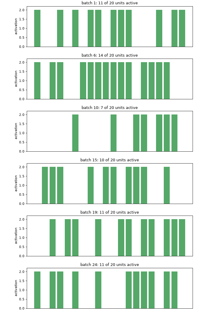A different thinned network on every batch.

In [10]:

dropout_results = {}
for p in [0.0, 0.2, 0.5]:
    torch.manual_seed(0)
    print(f'dropout p = {p}')
    dropout_results[p] = fit(MLP(dropout=p), epochs=40, verbose_every=40, label=f'p={p}')

plt.figure(figsize=(7, 4.5))
for p, hist in dropout_results.items():
    plt.plot(hist['val_acc'], label=f'dropout p = {p}')
plt.xlabel('Epoch'); plt.ylabel('Validation accuracy (%)')
plt.title('Dropout')
plt.legend(); plt.grid(alpha=0.3)
plt.show()

dropout_results = {} for p in [0.0, 0.2, 0.5]: torch.manual_seed(0) print(f'dropout p = {p}') dropout_results[p] = fit(MLP(dropout=p), epochs=40, verbose_every=40, label=f'p={p}') plt.figure(figsize=(7, 4.5)) for p, hist in dropout_results.items(): plt.plot(hist['val_acc'], label=f'dropout p = {p}') plt.xlabel('Epoch'); plt.ylabel('Validation accuracy (%)') plt.title('Dropout') plt.legend(); plt.grid(alpha=0.3) plt.show()

dropout p = 0.0

  [p=0.0] epoch  40  train 0.0173/ 99.6%  val 1.0356/ 82.9%
dropout p = 0.2

  [p=0.2] epoch  40  train 0.0775/ 97.2%  val 0.8394/ 83.2%
dropout p = 0.5

  [p=0.5] epoch  40  train 0.2192/ 92.7%  val 0.6015/ 84.9%

5. Batch Normalization¶

Batch normalization standardises each layer's inputs across the batch, then lets the network rescale them with two learned parameters $\gamma$ and $\beta$:

$$ \hat{x} = \frac{x - \mu_{\text{batch}}}{\sqrt{\sigma^2_{\text{batch}} + \epsilon}}, \qquad y = \gamma \hat{x} + \beta $$

It was introduced to fix "internal covariate shift"; the current understanding is that its main effect is to smooth the loss landscape, which lets you train faster and with higher learning rates. It also has a mild regularizing side effect, because each sample's normalisation depends on whichever other samples landed in its batch.

Like dropout, it behaves differently in the two modes: during training it uses the batch statistics, during evaluation it uses running averages accumulated over training. That is the second reason model.eval() matters.

In [11]:

bn_results = {}
for use_bn in [False, True]:
    torch.manual_seed(0)
    print(f'batchnorm = {use_bn}')
    bn_results[use_bn] = fit(MLP(batchnorm=use_bn), epochs=40,
                             verbose_every=40, label=f'bn={use_bn}')

plt.figure(figsize=(7, 4.5))
for use_bn, hist in bn_results.items():
    plt.plot(hist['val_acc'], label=f'batchnorm = {use_bn}')
plt.xlabel('Epoch'); plt.ylabel('Validation accuracy (%)')
plt.title('Batch normalization: mainly faster convergence')
plt.legend(); plt.grid(alpha=0.3)
plt.show()

bn_results = {} for use_bn in [False, True]: torch.manual_seed(0) print(f'batchnorm = {use_bn}') bn_results[use_bn] = fit(MLP(batchnorm=use_bn), epochs=40, verbose_every=40, label=f'bn={use_bn}') plt.figure(figsize=(7, 4.5)) for use_bn, hist in bn_results.items(): plt.plot(hist['val_acc'], label=f'batchnorm = {use_bn}') plt.xlabel('Epoch'); plt.ylabel('Validation accuracy (%)') plt.title('Batch normalization: mainly faster convergence') plt.legend(); plt.grid(alpha=0.3) plt.show()

batchnorm = False

  [bn=False] epoch  40  train 0.0173/ 99.6%  val 1.0356/ 82.9%
batchnorm = True

  [bn=True] epoch  40  train 0.0540/ 98.3%  val 0.8355/ 82.7%

6. Data Augmentation¶

The other way to fix overfitting is the direct one: get more data. Augmentation fakes it, by applying label-preserving transformations — a flipped shirt is still a shirt.

Augmentation is applied on the fly, so the network sees a slightly different version of every image at every epoch. Unlike the other techniques it costs no model capacity, and on image tasks it is often the strongest regularizer available.

"Often" is doing real work in that sentence, so we are going to test it rather than repeat it. Two candidate policies:

• flip only — a horizontal mirror.
• flip + affine — mirror, plus small rotations, shifts and rescaling. The more thorough-looking option, and the one most tutorials reach for.

Choose transformations to match the domain. Horizontal flips suit clothing; they are wrong for digits (a mirrored 2 is not a 2) and wrong for text.

In [12]:

flip_tf = transforms.Compose([
    transforms.RandomHorizontalFlip(),
    transforms.ToTensor(),
    transforms.Normalize((0.2860,), (0.3530,)),
])

strong_tf = transforms.Compose([
    transforms.RandomHorizontalFlip(),
    transforms.RandomAffine(degrees=10, translate=(0.1, 0.1), scale=(0.9, 1.1)),
    transforms.ToTensor(),
    transforms.Normalize((0.2860,), (0.3530,)),
])

def subset_with(tf):
    return Subset(datasets.FashionMNIST(root='./data', train=True, download=True,
                                        transform=tf), range(N_TRAIN))

flip_train, strong_train = subset_with(flip_tf), subset_with(strong_tf)

# The same source image, eight times, under each policy
fig, axes = plt.subplots(2, 8, figsize=(11, 3))
for row, (dataset, name) in enumerate([(flip_train, 'flip'), (strong_train, 'flip + affine')]):
    for ax in axes[row]:
        img, lab = dataset[0]
        ax.imshow(img[0], cmap='gray')
        ax.axis('off')
    axes[row, 0].set_title(name, loc='left', fontsize=9)
fig.suptitle(f'One "{CLASSES[flip_train[0][1]]}" image, resampled', fontsize=10)
plt.tight_layout()
plt.show()

flip_tf = transforms.Compose([ transforms.RandomHorizontalFlip(), transforms.ToTensor(), transforms.Normalize((0.2860,), (0.3530,)), ]) strong_tf = transforms.Compose([ transforms.RandomHorizontalFlip(), transforms.RandomAffine(degrees=10, translate=(0.1, 0.1), scale=(0.9, 1.1)), transforms.ToTensor(), transforms.Normalize((0.2860,), (0.3530,)), ]) def subset_with(tf): return Subset(datasets.FashionMNIST(root='./data', train=True, download=True, transform=tf), range(N_TRAIN)) flip_train, strong_train = subset_with(flip_tf), subset_with(strong_tf) # The same source image, eight times, under each policy fig, axes = plt.subplots(2, 8, figsize=(11, 3)) for row, (dataset, name) in enumerate([(flip_train, 'flip'), (strong_train, 'flip + affine')]): for ax in axes[row]: img, lab = dataset[0] ax.imshow(img[0], cmap='gray') ax.axis('off') axes[row, 0].set_title(name, loc='left', fontsize=9) fig.suptitle(f'One "{CLASSES[flip_train[0][1]]}" image, resampled', fontsize=10) plt.tight_layout() plt.show()

In [13]:

flip_loader = DataLoader(flip_train, batch_size=64, shuffle=True)
strong_loader = DataLoader(strong_train, batch_size=64, shuffle=True)

torch.manual_seed(0)
flip_hist = fit(MLP(), epochs=40, verbose_every=40, label='flip', loader=flip_loader)
torch.manual_seed(0)
strong_hist = fit(MLP(), epochs=40, verbose_every=40, label='flip+affine', loader=strong_loader)

plt.figure(figsize=(7, 4.5))
plt.plot(baseline['val_acc'], label='no augmentation')
plt.plot(flip_hist['val_acc'], label='flip only')
plt.plot(strong_hist['val_acc'], label='flip + affine')
plt.xlabel('Epoch'); plt.ylabel('Validation accuracy (%)')
plt.title('Not all augmentation helps')
plt.legend(); plt.grid(alpha=0.3)
plt.show()

for name, hist in [('none', baseline), ('flip only', flip_hist), ('flip + affine', strong_hist)]:
    print(f'  {name:14s} best val acc {max(hist["val_acc"]):.2f}%   '
          f'final train acc {hist["train_acc"][-1]:.2f}%')

flip_loader = DataLoader(flip_train, batch_size=64, shuffle=True) strong_loader = DataLoader(strong_train, batch_size=64, shuffle=True) torch.manual_seed(0) flip_hist = fit(MLP(), epochs=40, verbose_every=40, label='flip', loader=flip_loader) torch.manual_seed(0) strong_hist = fit(MLP(), epochs=40, verbose_every=40, label='flip+affine', loader=strong_loader) plt.figure(figsize=(7, 4.5)) plt.plot(baseline['val_acc'], label='no augmentation') plt.plot(flip_hist['val_acc'], label='flip only') plt.plot(strong_hist['val_acc'], label='flip + affine') plt.xlabel('Epoch'); plt.ylabel('Validation accuracy (%)') plt.title('Not all augmentation helps') plt.legend(); plt.grid(alpha=0.3) plt.show() for name, hist in [('none', baseline), ('flip only', flip_hist), ('flip + affine', strong_hist)]: print(f' {name:14s} best val acc {max(hist["val_acc"]):.2f}% ' f'final train acc {hist["train_acc"][-1]:.2f}%')

  [flip] epoch  40  train 0.1284/ 95.7%  val 0.7904/ 83.2%

  [flip+affine] epoch  40  train 0.5152/ 79.8%  val 0.6250/ 77.7%

  none           best val acc 83.50%   final train acc 99.60%
  flip only      best val acc 84.15%   final train acc 95.65%
  flip + affine  best val acc 79.55%   final train acc 79.85%

The flip helps a little. The thorough-looking option makes things clearly worse.

That is not a bug, and it is worth understanding rather than tuning away. The affine transform shifts, rotates and rescales 28x28 images in which the garment already fills the frame, so it pushes pixels off the edge and pads the gap. The training distribution drifts away from the test distribution, which is not augmented — and with only 2,000 images and 40 epochs, the network never gets enough passes to benefit from the extra variety it does provide.

Two lessons, both general:

1. Augmentation strength is a hyperparameter, with the same too-little/too-much curve as weight decay and dropout. "More augmentation" is not a safe default.
2. Augmentation interacts with the training budget. Aggressive transforms make each epoch harder, so they need more epochs to pay off. Judging them at a budget tuned for the un-augmented baseline is judging them unfairly — and doing so is the single most common way this comparison is gotten wrong.

We carry the flip-only policy forward, because it is the one that actually helped.

In [14]:

augmented_loader = flip_loader      # the policy that survived the comparison
aug_hist = flip_hist

augmented_loader = flip_loader # the policy that survived the comparison aug_hist = flip_hist

7. Early Stopping¶

The cheapest regularizer of all: notice when validation loss stops improving, and stop.

The implementation detail that matters is that you must keep the best weights, not the last ones. Training past the optimum and then stopping leaves you with a worse model than the one you already had.

In [15]:

import copy

def fit_with_early_stopping(model, epochs=60, lr=1e-3, patience=8, label=''):
    model = model.to(device)
    optimizer = optim.Adam(model.parameters(), lr=lr)
    best_loss, best_state, best_epoch, waited = float('inf'), None, 0, 0
    hist = {'train_loss': [], 'val_loss': [], 'val_acc': []}

    for epoch in range(epochs):
        tr_loss, _ = run_epoch(model, train_loader, optimizer)
        va_loss, va_acc = run_epoch(model, val_loader)
        hist['train_loss'].append(tr_loss)
        hist['val_loss'].append(va_loss)
        hist['val_acc'].append(va_acc)

        if va_loss < best_loss:
            best_loss, best_epoch, waited = va_loss, epoch, 0
            best_state = copy.deepcopy(model.state_dict())   # keep the good weights
        else:
            waited += 1
            if waited >= patience:
                print(f'  [{label}] no improvement for {patience} epochs - stopping at {epoch+1}')
                break

    model.load_state_dict(best_state)                        # roll back to the best
    print(f'  [{label}] best epoch was {best_epoch + 1} '
          f'(val loss {best_loss:.4f}, val acc {hist["val_acc"][best_epoch]:.2f}%)')
    return model, hist, best_epoch

torch.manual_seed(0)
es_model, es_hist, es_best = fit_with_early_stopping(MLP(), label='early stop')

plt.figure(figsize=(7, 4.5))
plt.plot(es_hist['train_loss'], label='train loss')
plt.plot(es_hist['val_loss'], label='validation loss')
plt.axvline(es_best, color='gray', linestyle='--', label=f'restored epoch {es_best + 1}')
plt.xlabel('Epoch'); plt.ylabel('Loss')
plt.title('Early stopping keeps the best weights, not the last')
plt.legend(); plt.grid(alpha=0.3)
plt.show()

import copy def fit_with_early_stopping(model, epochs=60, lr=1e-3, patience=8, label=''): model = model.to(device) optimizer = optim.Adam(model.parameters(), lr=lr) best_loss, best_state, best_epoch, waited = float('inf'), None, 0, 0 hist = {'train_loss': [], 'val_loss': [], 'val_acc': []} for epoch in range(epochs): tr_loss, _ = run_epoch(model, train_loader, optimizer) va_loss, va_acc = run_epoch(model, val_loader) hist['train_loss'].append(tr_loss) hist['val_loss'].append(va_loss) hist['val_acc'].append(va_acc) if va_loss < best_loss: best_loss, best_epoch, waited = va_loss, epoch, 0 best_state = copy.deepcopy(model.state_dict()) # keep the good weights else: waited += 1 if waited >= patience: print(f' [{label}] no improvement for {patience} epochs - stopping at {epoch+1}') break model.load_state_dict(best_state) # roll back to the best print(f' [{label}] best epoch was {best_epoch + 1} ' f'(val loss {best_loss:.4f}, val acc {hist["val_acc"][best_epoch]:.2f}%)') return model, hist, best_epoch torch.manual_seed(0) es_model, es_hist, es_best = fit_with_early_stopping(MLP(), label='early stop') plt.figure(figsize=(7, 4.5)) plt.plot(es_hist['train_loss'], label='train loss') plt.plot(es_hist['val_loss'], label='validation loss') plt.axvline(es_best, color='gray', linestyle='--', label=f'restored epoch {es_best + 1}') plt.xlabel('Epoch'); plt.ylabel('Loss') plt.title('Early stopping keeps the best weights, not the last') plt.legend(); plt.grid(alpha=0.3) plt.show()

  [early stop] no improvement for 8 epochs - stopping at 16
  [early stop] best epoch was 8 (val loss 0.5363, val acc 82.35%)

8. Optimizers: How the Weights Actually Move¶

Regularization decides what the network is allowed to learn. The optimizer decides how it gets there.

All of them descend the gradient; they differ in how much history they use:

• SGD steps straight downhill: $w \leftarrow w - \eta \nabla \mathcal{L}$. Simple, and it oscillates badly in valleys that are steep in one direction and shallow in another.
• SGD with momentum accumulates a velocity, so consistent directions build up speed and oscillations cancel out.
• RMSprop keeps a running average of squared gradients and divides by it, giving each parameter its own effective step size.
• Adam combines both: momentum and per-parameter scaling. It is the sensible default, which is why every lab so far has used it.

The classic test case is a "ravine" — $f(x, y) = x^2/20 + y^2$ — steep across, shallow along. Watch how differently the four optimizers handle it.

In [16]:

def optimize_path(make_opt, start=(-7.0, 2.5), steps=90):
    """Run a real torch optimizer on f(x, y) = x^2/20 + y^2 and record the path."""
    p = torch.tensor(start, requires_grad=True)
    opt = make_opt([p])
    path = [p.detach().clone().numpy()]
    for _ in range(steps):
        loss = p[0] ** 2 / 20 + p[1] ** 2
        opt.zero_grad()
        loss.backward()
        opt.step()
        path.append(p.detach().clone().numpy())
    return np.array(path)

runs = {
    'SGD (lr=0.4)': (optimize_path(lambda p: optim.SGD(p, lr=0.4)), '#C44E52'),
    'Momentum (0.9)': (optimize_path(lambda p: optim.SGD(p, lr=0.4, momentum=0.9)), '#DD8452'),
    'RMSprop (lr=0.4)': (optimize_path(lambda p: optim.RMSprop(p, lr=0.4)), '#55A868'),
    'Adam (lr=0.4)': (optimize_path(lambda p: optim.Adam(p, lr=0.4)), '#4C72B0'),
}

xs = np.linspace(-9, 9, 300)
ys = np.linspace(-4, 4, 200)
XX, YY = np.meshgrid(xs, ys)
ZZ = XX ** 2 / 20 + YY ** 2

fig, ax = plt.subplots(figsize=(9, 4.2))
ax.contour(XX, YY, ZZ, levels=np.logspace(-1.5, 2, 18), cmap='Greys', linewidths=0.7)
ax.plot(0, 0, '*', color='gold', markersize=16, markeredgecolor='k', label='minimum')

lines, heads = {}, {}
for name, (path, color) in runs.items():
    lines[name], = ax.plot([], [], color=color, lw=1.8, label=name)
    heads[name], = ax.plot([], [], 'o', color=color, markersize=6)
ax.set_xlim(-9, 9); ax.set_ylim(-4, 4)
ax.legend(loc='upper right', fontsize=8)
ax.set_title('Four optimizers on the same ravine')

def update(k):
    for name, (path, _) in runs.items():
        lines[name].set_data(path[:k + 1, 0], path[:k + 1, 1])
        heads[name].set_data([path[k, 0]], [path[k, 1]])
    return list(lines.values()) + list(heads.values())

ani = animation.FuncAnimation(fig, update, frames=len(next(iter(runs.values()))[0]),
                              interval=70, blit=False)
plt.close(fig)
save_animation(ani, 'lab13_optimizers.gif', fps=14)

def optimize_path(make_opt, start=(-7.0, 2.5), steps=90): """Run a real torch optimizer on f(x, y) = x^2/20 + y^2 and record the path.""" p = torch.tensor(start, requires_grad=True) opt = make_opt([p]) path = [p.detach().clone().numpy()] for _ in range(steps): loss = p[0] ** 2 / 20 + p[1] ** 2 opt.zero_grad() loss.backward() opt.step() path.append(p.detach().clone().numpy()) return np.array(path) runs = { 'SGD (lr=0.4)': (optimize_path(lambda p: optim.SGD(p, lr=0.4)), '#C44E52'), 'Momentum (0.9)': (optimize_path(lambda p: optim.SGD(p, lr=0.4, momentum=0.9)), '#DD8452'), 'RMSprop (lr=0.4)': (optimize_path(lambda p: optim.RMSprop(p, lr=0.4)), '#55A868'), 'Adam (lr=0.4)': (optimize_path(lambda p: optim.Adam(p, lr=0.4)), '#4C72B0'), } xs = np.linspace(-9, 9, 300) ys = np.linspace(-4, 4, 200) XX, YY = np.meshgrid(xs, ys) ZZ = XX ** 2 / 20 + YY ** 2 fig, ax = plt.subplots(figsize=(9, 4.2)) ax.contour(XX, YY, ZZ, levels=np.logspace(-1.5, 2, 18), cmap='Greys', linewidths=0.7) ax.plot(0, 0, '*', color='gold', markersize=16, markeredgecolor='k', label='minimum') lines, heads = {}, {} for name, (path, color) in runs.items(): lines[name], = ax.plot([], [], color=color, lw=1.8, label=name) heads[name], = ax.plot([], [], 'o', color=color, markersize=6) ax.set_xlim(-9, 9); ax.set_ylim(-4, 4) ax.legend(loc='upper right', fontsize=8) ax.set_title('Four optimizers on the same ravine') def update(k): for name, (path, _) in runs.items(): lines[name].set_data(path[:k + 1, 0], path[:k + 1, 1]) heads[name].set_data([path[k, 0]], [path[k, 1]]) return list(lines.values()) + list(heads.values()) ani = animation.FuncAnimation(fig, update, frames=len(next(iter(runs.values()))[0]), interval=70, blit=False) plt.close(fig) save_animation(ani, 'lab13_optimizers.gif', fps=14)

saved Misc\lab13_optimizers.gif  (0.5 MB)

Out[16]:

'Misc\\lab13_optimizers.gif'

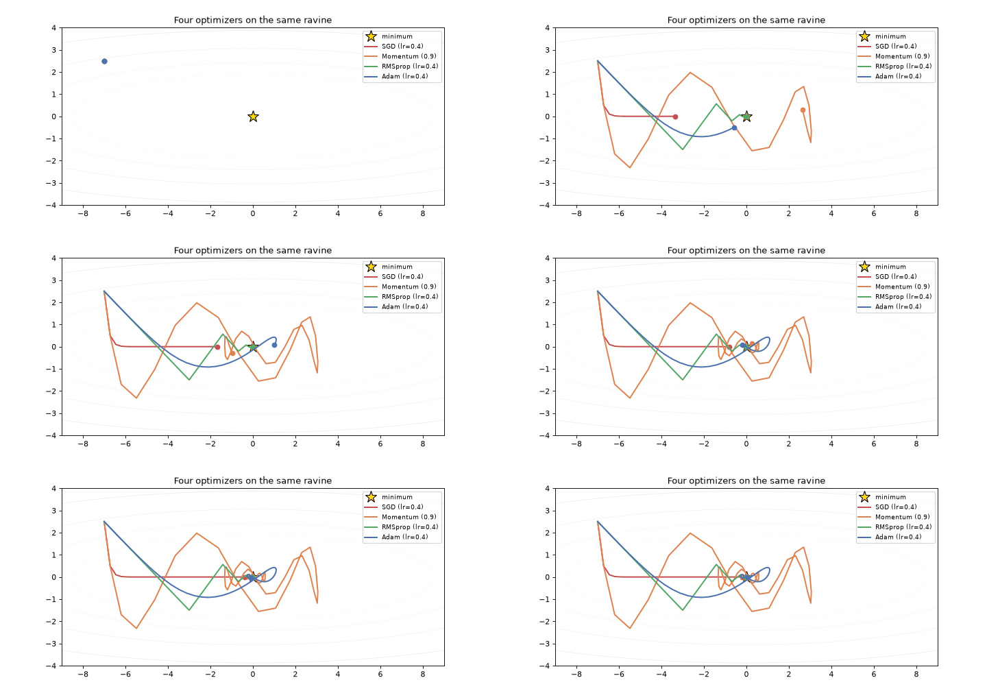Four optimizers descending the same ravine. SGD zigzags; Adam goes almost straight in.

SGD zigzags across the steep axis and crawls along the shallow one. Momentum damps the zigzag and picks up speed. RMSprop and Adam rescale each axis and go almost straight in.

This is a two-parameter toy, and real loss surfaces are not so tidy — but the intuition holds, and it explains why Adam is the safe default when you have no time to tune.

9. The Learning Rate, and How to Schedule It¶

If you can only tune one hyperparameter, tune this one.

• Too small: training crawls, and can stall in a bad region.
• Too large: updates overshoot, the loss oscillates or diverges to nan.
• About right: fast progress at first, then it needs to shrink to settle into a minimum.

That last point is why schedules exist: start high to cover ground, end low to converge. StepLR drops by a factor every few epochs; CosineAnnealingLR decays smoothly to zero; OneCycleLR warms up and then anneals, which is what most modern recipes use.

In [17]:

for lr in [1e-1, 1e-2, 1e-3, 1e-4]:
    torch.manual_seed(0)
    h = fit(MLP(), epochs=12, lr=lr, verbose_every=0)
    print(f'lr = {lr:<7} final train loss {h["train_loss"][-1]:8.4f}   '
          f'best val acc {max(h["val_acc"]):.2f}%')

for lr in [1e-1, 1e-2, 1e-3, 1e-4]: torch.manual_seed(0) h = fit(MLP(), epochs=12, lr=lr, verbose_every=0) print(f'lr = {lr:<7} final train loss {h["train_loss"][-1]:8.4f} ' f'best val acc {max(h["val_acc"]):.2f}%')

lr = 0.1     final train loss   2.3093   best val acc 27.40%

lr = 0.01    final train loss   0.4617   best val acc 80.50%

lr = 0.001   final train loss   0.1716   best val acc 83.00%

lr = 0.0001  final train loss   0.3631   best val acc 82.30%

In [18]:

# What the schedules look like
demo = nn.Linear(1, 1)
schedules = {
    'constant': lambda o: optim.lr_scheduler.ConstantLR(o, factor=1.0, total_iters=1),
    'StepLR (x0.5 every 10)': lambda o: optim.lr_scheduler.StepLR(o, step_size=10, gamma=0.5),
    'ExponentialLR (0.93)': lambda o: optim.lr_scheduler.ExponentialLR(o, gamma=0.93),
    'CosineAnnealingLR': lambda o: optim.lr_scheduler.CosineAnnealingLR(o, T_max=40),
}

plt.figure(figsize=(7, 4))
for name, make in schedules.items():
    opt = optim.Adam(demo.parameters(), lr=1e-2)
    sched = make(opt)
    trace = []
    for _ in range(40):
        trace.append(opt.param_groups[0]['lr'])
        opt.step()
        sched.step()
    plt.plot(trace, label=name)
plt.xlabel('Epoch'); plt.ylabel('Learning rate')
plt.title('Learning rate schedules')
plt.legend(fontsize=8); plt.grid(alpha=0.3)
plt.show()

# What the schedules look like demo = nn.Linear(1, 1) schedules = { 'constant': lambda o: optim.lr_scheduler.ConstantLR(o, factor=1.0, total_iters=1), 'StepLR (x0.5 every 10)': lambda o: optim.lr_scheduler.StepLR(o, step_size=10, gamma=0.5), 'ExponentialLR (0.93)': lambda o: optim.lr_scheduler.ExponentialLR(o, gamma=0.93), 'CosineAnnealingLR': lambda o: optim.lr_scheduler.CosineAnnealingLR(o, T_max=40), } plt.figure(figsize=(7, 4)) for name, make in schedules.items(): opt = optim.Adam(demo.parameters(), lr=1e-2) sched = make(opt) trace = [] for _ in range(40): trace.append(opt.param_groups[0]['lr']) opt.step() sched.step() plt.plot(trace, label=name) plt.xlabel('Epoch'); plt.ylabel('Learning rate') plt.title('Learning rate schedules') plt.legend(fontsize=8); plt.grid(alpha=0.3) plt.show()

In [19]:

torch.manual_seed(0)
cos_hist = fit(MLP(), epochs=40, lr=1e-3,
               scheduler_fn=lambda o: optim.lr_scheduler.CosineAnnealingLR(o, T_max=40),
               verbose_every=20, label='cosine')

fig, (ax1, ax2) = plt.subplots(1, 2, figsize=(11, 4))
ax1.plot(baseline['val_acc'], label='constant lr')
ax1.plot(cos_hist['val_acc'], label='cosine schedule')
ax1.set_xlabel('Epoch'); ax1.set_ylabel('Validation accuracy (%)')
ax1.legend(); ax1.grid(alpha=0.3); ax1.set_title('Effect of the schedule')
ax2.plot(cos_hist['lr'], color='#8172B3')
ax2.set_xlabel('Epoch'); ax2.set_ylabel('Learning rate'); ax2.set_title('The schedule itself')
ax2.grid(alpha=0.3)
plt.tight_layout()
plt.show()

torch.manual_seed(0) cos_hist = fit(MLP(), epochs=40, lr=1e-3, scheduler_fn=lambda o: optim.lr_scheduler.CosineAnnealingLR(o, T_max=40), verbose_every=20, label='cosine') fig, (ax1, ax2) = plt.subplots(1, 2, figsize=(11, 4)) ax1.plot(baseline['val_acc'], label='constant lr') ax1.plot(cos_hist['val_acc'], label='cosine schedule') ax1.set_xlabel('Epoch'); ax1.set_ylabel('Validation accuracy (%)') ax1.legend(); ax1.grid(alpha=0.3); ax1.set_title('Effect of the schedule') ax2.plot(cos_hist['lr'], color='#8172B3') ax2.set_xlabel('Epoch'); ax2.set_ylabel('Learning rate'); ax2.set_title('The schedule itself') ax2.grid(alpha=0.3) plt.tight_layout() plt.show()

  [cosine] epoch  20  train 0.0569/ 98.2%  val 0.7912/ 83.5%

  [cosine] epoch  40  train 0.0038/100.0%  val 1.0034/ 84.0%

10. Putting It All Together¶

Each technique gave a modest improvement on its own. The natural next step is to switch them all on at once — so let's do exactly that, with the settings that worked individually, and see what happens.

In [20]:

torch.manual_seed(0)
naive_combined = fit(MLP(hidden=512, dropout=0.3, batchnorm=True),
                     epochs=60, lr=1e-3, weight_decay=1e-4,
                     scheduler_fn=lambda o: optim.lr_scheduler.CosineAnnealingLR(o, T_max=60),
                     verbose_every=30, label='naive combo',
                     loader=strong_loader)        # the aggressive augmentation

print(f'\nBaseline best      : {max(baseline["val_acc"]):.2f}%')
print(f'Everything at once : {max(naive_combined["val_acc"]):.2f}%')

torch.manual_seed(0) naive_combined = fit(MLP(hidden=512, dropout=0.3, batchnorm=True), epochs=60, lr=1e-3, weight_decay=1e-4, scheduler_fn=lambda o: optim.lr_scheduler.CosineAnnealingLR(o, T_max=60), verbose_every=30, label='naive combo', loader=strong_loader) # the aggressive augmentation print(f'\nBaseline best : {max(baseline["val_acc"]):.2f}%') print(f'Everything at once : {max(naive_combined["val_acc"]):.2f}%')

  [naive combo] epoch  30  train 0.6672/ 75.0%  val 0.5794/ 78.6%

  [naive combo] epoch  60  train 0.5601/ 78.5%  val 0.5381/ 80.2%

Baseline best      : 83.50%
Everything at once : 80.25%

Worse than the baseline. Switching on five regularizers that each helped alone produced a model worse than no regularization at all.

This is the most useful failure in the lab, because the reason is not exotic. Each technique was tuned in isolation, against a model that was overfitting badly. Applied together they do not add — they compound, and the model swings from overfitting to underfitting. Look back at section 3: weight decay at 0.1 dropped accuracy to 69%. Five mild constraints can add up to one severe one.

There is also a specific offender here, and section 6 already identified it: the aggressive flip + affine augmentation, which lost 4 points on its own at this budget.

So we retune, changing three things:

1. Milder augmentation. Keep the flip, shrink the affine, drop the rescaling.
2. Rebalance the constraints. Less dropout (0.2 rather than 0.3), more weight decay (1e-2 rather than 1e-4) — the value section 3 actually found best.
3. A longer budget. Augmented data makes every epoch harder, so it needs more epochs to pay off. This was lesson two from section 6, and here is where it gets tested.

In [21]:

mild_tf = transforms.Compose([
    transforms.RandomHorizontalFlip(),
    transforms.RandomAffine(degrees=6, translate=(0.06, 0.06)),   # gentler, no rescaling
    transforms.ToTensor(),
    transforms.Normalize((0.2860,), (0.3530,)),
])
mild_loader = DataLoader(subset_with(mild_tf), batch_size=64, shuffle=True)

torch.manual_seed(0)
combined_hist = fit(MLP(hidden=512, dropout=0.2, batchnorm=True),
                    epochs=120, lr=1e-3, weight_decay=1e-2,
                    scheduler_fn=lambda o: optim.lr_scheduler.CosineAnnealingLR(o, T_max=120),
                    verbose_every=40, label='retuned',
                    loader=mild_loader)

print(f'\nBaseline           : {max(baseline["val_acc"]):.2f}%')
print(f'Everything at once : {max(naive_combined["val_acc"]):.2f}%')
print(f'Retuned            : {max(combined_hist["val_acc"]):.2f}%')

mild_tf = transforms.Compose([ transforms.RandomHorizontalFlip(), transforms.RandomAffine(degrees=6, translate=(0.06, 0.06)), # gentler, no rescaling transforms.ToTensor(), transforms.Normalize((0.2860,), (0.3530,)), ]) mild_loader = DataLoader(subset_with(mild_tf), batch_size=64, shuffle=True) torch.manual_seed(0) combined_hist = fit(MLP(hidden=512, dropout=0.2, batchnorm=True), epochs=120, lr=1e-3, weight_decay=1e-2, scheduler_fn=lambda o: optim.lr_scheduler.CosineAnnealingLR(o, T_max=120), verbose_every=40, label='retuned', loader=mild_loader) print(f'\nBaseline : {max(baseline["val_acc"]):.2f}%') print(f'Everything at once : {max(naive_combined["val_acc"]):.2f}%') print(f'Retuned : {max(combined_hist["val_acc"]):.2f}%')

  [retuned] epoch  40  train 0.6733/ 77.3%  val 0.6271/ 78.2%

  [retuned] epoch  80  train 0.5376/ 82.2%  val 0.4777/ 84.2%

  [retuned] epoch 120  train 0.3795/ 87.7%  val 0.4378/ 85.5%

Baseline           : 83.50%
Everything at once : 80.25%
Retuned            : 85.90%

In [22]:

results = {
    'baseline': baseline,
    'weight decay 1e-2': wd_results[1e-2],
    'dropout 0.5': dropout_results[0.5],
    'batchnorm': bn_results[True],
    'flip augmentation': aug_hist,
    'cosine lr': cos_hist,
    'everything at once': naive_combined,
    'retuned combination': combined_hist,
}

print(f'{"configuration":24s} {"best":>7} {"final":>7} {"train":>7}   vs baseline')
print('-' * 66)
base_best = max(baseline['val_acc'])
for name, hist in results.items():
    best = max(hist['val_acc'])
    delta = best - base_best
    marker = '' if name == 'baseline' else f'{delta:+6.2f}'
    print(f'{name:24s} {best:>6.2f}% {hist["val_acc"][-1]:>6.2f}% '
          f'{hist["train_acc"][-1]:>6.2f}%   {marker}')

results = { 'baseline': baseline, 'weight decay 1e-2': wd_results[1e-2], 'dropout 0.5': dropout_results[0.5], 'batchnorm': bn_results[True], 'flip augmentation': aug_hist, 'cosine lr': cos_hist, 'everything at once': naive_combined, 'retuned combination': combined_hist, } print(f'{"configuration":24s} {"best":>7} {"final":>7} {"train":>7} vs baseline') print('-' * 66) base_best = max(baseline['val_acc']) for name, hist in results.items(): best = max(hist['val_acc']) delta = best - base_best marker = '' if name == 'baseline' else f'{delta:+6.2f}' print(f'{name:24s} {best:>6.2f}% {hist["val_acc"][-1]:>6.2f}% ' f'{hist["train_acc"][-1]:>6.2f}% {marker}')

configuration               best   final   train   vs baseline
------------------------------------------------------------------
baseline                  83.50%  82.90%  99.60%   
weight decay 1e-2         84.15%  81.85%  94.85%    +0.65
dropout 0.5               84.90%  84.90%  92.65%    +1.40
batchnorm                 83.65%  82.65%  98.30%    +0.15
flip augmentation         84.15%  83.20%  95.65%    +0.65
cosine lr                 84.25%  83.95%  99.95%    +0.75
everything at once        80.25%  80.20%  78.50%    -3.25
retuned combination       85.90%  85.55%  87.65%    +2.40

In [23]:

fig, (ax1, ax2) = plt.subplots(1, 2, figsize=(13, 4.5))
for name, hist in results.items():
    ax1.plot(hist['val_acc'], label=name,
             lw=2.2 if 'combination' in name else 1.1)
ax1.set_xlabel('Epoch'); ax1.set_ylabel('Validation accuracy (%)')
ax1.set_title('Every configuration, same axes')
ax1.legend(fontsize=8); ax1.grid(alpha=0.3)

names = list(results)
bests = [max(h['val_acc']) for h in results.values()]
colors = ['#C44E52' if b < base_best else '#4C72B0' for b in bests]
colors[0] = '#8172B3'
colors[-1] = '#55A868'
ax2.barh(names, bests, color=colors)
ax2.axvline(base_best, color='#8172B3', linestyle='--', lw=1, label='baseline')
ax2.set_xlim(min(bests) - 2, max(bests) + 1.5)
ax2.set_xlabel('Best validation accuracy (%)')
for i, v in enumerate(bests):
    ax2.text(v + 0.1, i, f'{v:.1f}', va='center', fontsize=9)
ax2.set_title('Red bars lost to doing nothing')
ax2.legend(fontsize=8)
plt.tight_layout()
plt.show()

gain = max(combined_hist['val_acc']) - base_best
print(f'Gain over baseline: {gain:+.2f} percentage points - same architecture, same 2,000 images.')

fig, (ax1, ax2) = plt.subplots(1, 2, figsize=(13, 4.5)) for name, hist in results.items(): ax1.plot(hist['val_acc'], label=name, lw=2.2 if 'combination' in name else 1.1) ax1.set_xlabel('Epoch'); ax1.set_ylabel('Validation accuracy (%)') ax1.set_title('Every configuration, same axes') ax1.legend(fontsize=8); ax1.grid(alpha=0.3) names = list(results) bests = [max(h['val_acc']) for h in results.values()] colors = ['#C44E52' if b < base_best else '#4C72B0' for b in bests] colors[0] = '#8172B3' colors[-1] = '#55A868' ax2.barh(names, bests, color=colors) ax2.axvline(base_best, color='#8172B3', linestyle='--', lw=1, label='baseline') ax2.set_xlim(min(bests) - 2, max(bests) + 1.5) ax2.set_xlabel('Best validation accuracy (%)') for i, v in enumerate(bests): ax2.text(v + 0.1, i, f'{v:.1f}', va='center', fontsize=9) ax2.set_title('Red bars lost to doing nothing') ax2.legend(fontsize=8) plt.tight_layout() plt.show() gain = max(combined_hist['val_acc']) - base_best print(f'Gain over baseline: {gain:+.2f} percentage points - same architecture, same 2,000 images.')

Gain over baseline: +2.40 percentage points - same architecture, same 2,000 images.

One honest caveat about these numbers. Every figure above is the best validation accuracy over training, and the retuned run had 120 epochs of chances at that maximum while the baseline had 40. Picking a maximum on the validation set is a mild form of fitting to it, and more epochs means more chances. Re-running the baseline at 120 epochs is the check that matters — it lands within a few tenths of its 40-epoch result, because it stopped improving long before, so the gain here is real. But the general habit is worth keeping: when you compare configurations, match the budget, and keep a test set you never look at.

11. Experiment: Try Different Settings¶

You can experiment with:

• Raising N_TRAIN to 10,000 and re-running the baseline — how much of the overfitting simply disappears?
• Swapping optim.Adam for optim.AdamW and comparing at the same weight_decay
• Adding nn.utils.clip_grad_norm_ via the clip argument of fit and pushing the learning rate higher than would otherwise be stable
• Replacing the cosine schedule with OneCycleLR (it steps per batch, not per epoch — you will need to move scheduler.step() inside the inner loop)
• Applying label smoothing: nn.CrossEntropyLoss(label_smoothing=0.1)
• Trying dropout at 0.7, or weight decay at 1.0, to see the underfitting side of the curve
• Running the whole comparison with a different random seed, to check which differences are real and which are noise

Try modifying the model definition or training loop above and observe how the performance changes.

12. Conclusion¶

In this lab, you learned the techniques that decide whether a network generalises. You provoked overfitting deliberately, then measured what each remedy actually bought — weight decay, dropout, batch normalization, augmentation and early stopping — and saw how optimizers and learning rate schedules change the path through the loss landscape.

Key takeaways:

• Diagnose from the gap between training and validation curves, not from either one alone.
• Every regularizer has a sweet spot: too little overfits, too much underfits.
• model.train() and model.eval() are not cosmetic — dropout and batch norm behave differently in each.
• Adam is a good default; momentum explains why it beats plain SGD in narrow valleys.
• Decay the learning rate. Almost every serious training run does.
• The techniques stack, and augmentation is usually the strongest one for images.

The next lab returns to architecture with the idea that replaced recurrence: attention.