Lab 14: Attention and Transformers
In Lab 11 you fixed the vanilla RNN's memory problem with gates. Attention takes a more radical approach: stop passing information along the sequence entirely. Instead, let every position look directly at every other position, in one step.
That single idea produced the Transformer, and with it essentially every large language model in use today.
We will cover the following topics:
- Why recurrence became the bottleneck
- Queries, keys and values, and scaled dot-product attention from scratch
- Multi-head attention, verified against
nn.MultiheadAttention - Positional encoding: putting order back into an order-blind model
- Building a Transformer encoder and training it on the task from Lab 11
- Reading the attention maps of the trained model
1. Why Replace Recurrence?
An LSTM carries information forward one step at a time. That has two costs:
- Path length. For position 60 to use information from position 1, the signal passes through 59 updates. The gates make that survivable, not free — and it still degrades with distance.
- No parallelism. Step $t$ cannot be computed until step $t-1$ is done. A 1,000-step sequence takes 1,000 sequential operations, no matter how many GPU cores you have. This is what limits training on long sequences, and it is the reason Transformers took over.
Attention removes both. Every position reaches every other position in one operation, and all positions are computed at the same time.
| RNN / LSTM | Attention | |
|---|---|---|
| Path between two positions | O(n) steps | O(1) steps |
| Parallel over the sequence | no | yes |
| Cost per layer | O(n · d²) | O(n² · d) |
| Handles long sequences | with difficulty | until n² becomes expensive |
The trade is visible in the last two rows: attention buys short paths and parallelism by comparing every pair of positions, which costs $n^2$.
2. Queries, Keys and Values
Attention is a soft dictionary lookup. Every position produces three vectors from its own embedding:
- a query $q$ — what am I looking for?
- a key $k$ — what do I offer?
- a value $v$ — what do I pass on if selected?
To compute the output for one position, we compare its query against every key, turn the resulting similarities into weights with a softmax, and take the weighted average of the values.

Written as one matrix expression over all positions at once:
$$ \text{Attention}(Q, K, V) = \text{softmax}\!\left(\frac{Q K^{\top}}{\sqrt{d_k}}\right) V $$
Why divide by $\sqrt{d_k}$? If the entries of $q$ and $k$ are roughly independent with unit variance, their dot product over $d_k$ dimensions has variance $d_k$ — so the scores grow with dimension. Large scores push softmax into a near one-hot regime where its gradient is almost zero, and training stalls. Dividing by $\sqrt{d_k}$ keeps the variance at 1 regardless of model size.
import math
import torch
import torch.nn as nn
import torch.optim as optim
import numpy as np
import matplotlib.pyplot as plt

torch.manual_seed(0)
device = torch.device('cuda' if torch.cuda.is_available() else 'cpu')
print('PyTorch version:', torch.__version__, '| device:', device)

def scaled_dot_product_attention(Q, K, V, mask=None):
    """Q, K, V: (..., seq_len, d_k). Returns the output and the attention weights."""
    d_k = Q.size(-1)
    scores = Q @ K.transpose(-2, -1) / math.sqrt(d_k)       # (..., seq_q, seq_k)
    if mask is not None:
        scores = scores.masked_fill(mask == 0, float('-inf'))
    weights = torch.softmax(scores, dim=-1)                  # each row sums to 1
    return weights @ V, weights

# A tiny worked example: 4 positions, 8 dimensions
seq_len, d_k = 4, 8
Q = torch.randn(seq_len, d_k)
K = torch.randn(seq_len, d_k)
V = torch.randn(seq_len, d_k)

out, attn = scaled_dot_product_attention(Q, K, V)
print('output shape    :', tuple(out.shape))
print('attention shape :', tuple(attn.shape), '  (one row of weights per query)')
print('rows sum to 1   :', attn.sum(dim=-1).detach().numpy().round(4))
PyTorch version: 2.13.0+cpu | device: cpu
output shape    : (4, 8)
attention shape : (4, 4)   (one row of weights per query)
rows sum to 1   : [1. 1. 1. 1.]
Seeing the scaling problem for yourself
The $\sqrt{d_k}$ term looks like a detail. It is not. Here is the same softmax with and without it, as the dimension grows.
print(f'{"d_k":>6} | {"max weight unscaled":>20} | {"max weight scaled":>18}')
print('-' * 52)
for d in [8, 64, 512, 4096]:
    q = torch.randn(1, d)
    k = torch.randn(16, d)
    unscaled = torch.softmax(q @ k.T, dim=-1).max().item()
    scaled = torch.softmax(q @ k.T / math.sqrt(d), dim=-1).max().item()
    print(f'{d:>6} | {unscaled:>20.4f} | {scaled:>18.4f}')
print('\nUnscaled, the softmax saturates towards one-hot as d_k grows - and a saturated')
print('softmax has almost no gradient, so the layer stops learning.')
   d_k |  max weight unscaled |  max weight scaled
----------------------------------------------------
     8 |               0.6302 |             0.1969
    64 |               0.7270 |             0.1527
   512 |               1.0000 |             0.2190
  4096 |               1.0000 |             0.4201

Unscaled, the softmax saturates towards one-hot as d_k grows - and a saturated
softmax has almost no gradient, so the layer stops learning.
3. Self-Attention and Masking
In self-attention, $Q$, $K$ and $V$ all come from the same sequence: every position attends to the sequence it belongs to, including itself. (In cross-attention, used by decoders, the queries come from one sequence and the keys and values from another.)
Sometimes we must forbid certain connections. A language model predicting the next token must not look at future tokens — that would be reading the answer. A causal mask zeroes out everything above the diagonal, so position $t$ can only attend to positions $\le t$.
n = 6
causal_mask = torch.tril(torch.ones(n, n))       # 1 = allowed, 0 = blocked
print('Causal mask (1 = may attend):')
print(causal_mask.int().numpy())

Q = torch.randn(n, 16)
K = torch.randn(n, 16)
V = torch.randn(n, 16)
_, attn_free = scaled_dot_product_attention(Q, K, V)
_, attn_causal = scaled_dot_product_attention(Q, K, V, mask=causal_mask)

fig, axes = plt.subplots(1, 2, figsize=(9, 3.6))
for ax, data, title in zip(axes, [attn_free, attn_causal],
                           ['unmasked (encoder)', 'causally masked (decoder)']):
    im = ax.imshow(data.detach().numpy(), cmap='viridis', vmin=0, vmax=1)
    ax.set_title(title, fontsize=10)
    ax.set_xlabel('key position (attended to)')
    ax.set_ylabel('query position')
    fig.colorbar(im, ax=ax, fraction=0.046)
plt.tight_layout()
plt.show()
Causal mask (1 = may attend):
[[1 0 0 0 0 0]
 [1 1 0 0 0 0]
 [1 1 1 0 0 0]
 [1 1 1 1 0 0]
 [1 1 1 1 1 0]
 [1 1 1 1 1 1]]

4. Multi-Head Attention
One attention operation produces one weighted average — a single notion of "relevant". Real relationships come in kinds: a word may relate to another as its subject, its modifier, or simply as the nearest noun.
Multi-head attention runs $h$ attention operations in parallel on different learned projections of the same input, each with dimension $d_{model}/h$, then concatenates the results and mixes them with one more linear layer:
$$ \text{MultiHead}(Q, K, V) = \text{Concat}(\text{head}_1, \ldots, \text{head}_h)\, W^O, \qquad \text{head}_i = \text{Attention}(Q W_i^Q,\, K W_i^K,\, V W_i^V) $$
Note that the total compute is unchanged: $h$ heads of size $d_{model}/h$ cost the same as one head of size $d_{model}$. Heads are free; you get them by reshaping.
Let's implement it and check against PyTorch, using the same borrow-the-weights trick as the RNN and LSTM labs.
embed_dim, num_heads, seq_len, batch = 32, 4, 6, 2
head_dim = embed_dim // num_heads

torch_mha = nn.MultiheadAttention(embed_dim, num_heads, batch_first=True)
x = torch.randn(batch, seq_len, embed_dim)

def manual_multihead(x, mha):
    """Multi-head self-attention written out, borrowing PyTorch's weights."""
    B, S, E = x.shape
    H = mha.num_heads
    D = E // H

    # PyTorch packs the three input projections into one (3E, E) matrix
    qkv = x @ mha.in_proj_weight.T + mha.in_proj_bias          # (B, S, 3E)
    Q, K, V = qkv.chunk(3, dim=-1)

    # split the embedding across heads: (B, S, E) -> (B, H, S, D)
    def split(t):
        return t.view(B, S, H, D).transpose(1, 2)
    Q, K, V = split(Q), split(K), split(V)

    out, weights = scaled_dot_product_attention(Q, K, V)       # per-head attention
    out = out.transpose(1, 2).reshape(B, S, E)                 # concatenate the heads
    out = mha.out_proj(out)                                    # final mix
    return out, weights

manual_out, per_head_weights = manual_multihead(x, torch_mha)
torch_out, torch_weights = torch_mha(x, x, x, need_weights=True)

print('manual output shape :', tuple(manual_out.shape))
print('per-head weights    :', tuple(per_head_weights.shape), '(batch, heads, query, key)')
print('outputs match       :', torch.allclose(manual_out, torch_out, atol=1e-5))
print('\nNote: nn.MultiheadAttention averages the heads in its returned weights by default;')
print('pass average_attn_weights=False to get them per head.')
manual output shape : (2, 6, 32)
per-head weights    : (2, 4, 6, 6) (batch, heads, query, key)
outputs match       : True

Note: nn.MultiheadAttention averages the heads in its returned weights by default;
pass average_attn_weights=False to get them per head.
The heads really do learn different things
Even at initialisation the four heads produce visibly different attention patterns, because their projections differ. After training, those differences become meaningful.
w = per_head_weights[0].detach().numpy()     # (heads, query, key)
fig, axes = plt.subplots(1, num_heads, figsize=(3 * num_heads, 3))
for h, ax in enumerate(axes):
    im = ax.imshow(w[h], cmap='viridis', vmin=0, vmax=w.max())
    ax.set_title(f'head {h + 1}', fontsize=10)
    ax.set_xlabel('key')
    if h == 0:
        ax.set_ylabel('query')
fig.suptitle('Four heads, four different views of the same sequence')
plt.tight_layout()
plt.show()

5. Positional Encoding
Attention has a property that is easy to miss: it is permutation equivariant. Shuffle the input positions and the outputs shuffle with them, unchanged. The mechanism has no notion of order at all — there is no "previous step" like in an RNN.
For most sequence tasks that is fatal, so we add position information directly to the embeddings. The original Transformer uses fixed sinusoids of geometrically spaced frequencies:
$$ PE_{(pos, 2i)} = \sin\!\left(\frac{pos}{10000^{2i/d_{model}}}\right), \qquad PE_{(pos, 2i+1)} = \cos\!\left(\frac{pos}{10000^{2i/d_{model}}}\right) $$
Each position gets a unique pattern across the embedding dimensions, fast-changing in the low dimensions and slow-changing in the high ones — like the digits of a binary counter, but continuous. Two useful properties follow: it extrapolates to sequences longer than any seen in training, and relative offsets are expressible as a fixed linear transform.
class PositionalEncoding(nn.Module):
    def __init__(self, d_model, max_len=512):
        super(PositionalEncoding, self).__init__()
        pe = torch.zeros(max_len, d_model)
        position = torch.arange(max_len).unsqueeze(1).float()
        div_term = torch.exp(torch.arange(0, d_model, 2).float()
                             * (-math.log(10000.0) / d_model))
        pe[:, 0::2] = torch.sin(position * div_term)
        pe[:, 1::2] = torch.cos(position * div_term)
        # register_buffer: saved with the model, but not a trainable parameter
        self.register_buffer('pe', pe.unsqueeze(0))

    def forward(self, x):
        return x + self.pe[:, :x.size(1)]

pos_enc = PositionalEncoding(d_model=64, max_len=100)
pe = pos_enc.pe[0].numpy()

fig, (ax1, ax2) = plt.subplots(1, 2, figsize=(11, 3.6))
im = ax1.imshow(pe.T, cmap='RdBu', aspect='auto')
ax1.set_xlabel('position'); ax1.set_ylabel('embedding dimension')
ax1.set_title('The positional encoding matrix')
fig.colorbar(im, ax=ax1, fraction=0.046)

for d in [0, 4, 12, 30]:
    ax2.plot(pe[:, d], label=f'dim {d}')
ax2.set_xlabel('position'); ax2.set_title('Low dimensions oscillate fast, high ones slow')
ax2.legend(fontsize=8); ax2.grid(alpha=0.3)
plt.tight_layout()
plt.show()

6. The Transformer Encoder Block
One encoder block is just two sub-layers, each wrapped in a residual connection and a layer normalization:

- Multi-head self-attention — positions exchange information.
- A position-wise feed-forward network — each position is processed independently, usually expanding to 4x the width and back.
The wrapping matters as much as the contents. The residual connections give gradients a direct path to every layer (the same additive trick that saves the LSTM's cell state), and layer normalization keeps activations at a stable scale. Stack a few of these and you have a Transformer encoder.
class EncoderBlock(nn.Module):
    def __init__(self, d_model, num_heads, ff_dim=None, dropout=0.1):
        super(EncoderBlock, self).__init__()
        ff_dim = ff_dim or 4 * d_model
        self.attn = nn.MultiheadAttention(d_model, num_heads,
                                          dropout=dropout, batch_first=True)
        self.norm1 = nn.LayerNorm(d_model)
        self.norm2 = nn.LayerNorm(d_model)
        self.ff = nn.Sequential(
            nn.Linear(d_model, ff_dim),
            nn.GELU(),
            nn.Dropout(dropout),
            nn.Linear(ff_dim, d_model),
        )
        self.dropout = nn.Dropout(dropout)

    def forward(self, x, need_weights=False):
        # pre-norm: normalise before each sub-layer, add the residual after
        h = self.norm1(x)
        attn_out, weights = self.attn(h, h, h,               # self-attention: Q = K = V
                                      need_weights=need_weights,
                                      average_attn_weights=False)
        x = x + self.dropout(attn_out)
        x = x + self.dropout(self.ff(self.norm2(x)))
        return (x, weights) if need_weights else (x, None)

block = EncoderBlock(d_model=32, num_heads=4)
sample = torch.randn(2, 10, 32)
out, _ = block(sample)
print('Block input :', tuple(sample.shape))
print('Block output:', tuple(out.shape), '- shape preserved, so blocks stack freely')
print(f'Parameters per block: {sum(p.numel() for p in block.parameters()):,}')
Block input : (2, 10, 32)
Block output: (2, 10, 32) - shape preserved, so blocks stack freely
Parameters per block: 12,704
Pre-norm vs post-norm: the 2017 paper applied layer norm after each residual addition. Practice has moved to normalising before the sub-layer, as above, because it trains far more stably at depth without a learning-rate warmup. Both work; pre-norm is the safer default.
7. Training a Transformer on the Lab 11 Task
Time for a fair comparison. We reuse the exact task from Lab 11 — a marker in the first position followed by 59 steps of noise, where only that marker decides the label.
Lab 11 showed that this task is solvable by a recurrent network, but delicately so: the vanilla RNN managed it, and the LSTM failed outright until its forget gate was initialised open. The difficulty is entirely about carrying one bit across 60 sequential updates.
Attention does not have that problem. The path from position 1 to the output is a single hop, no matter how long the sequence is, so none of the initialisation care that Lab 11 needed applies here.
We prepend a learned [CLS] token — a slot with no input of its own whose only job is to gather information for the classification. Its attention weights then show us, directly, which positions the model decided to read.
from torch.utils.data import TensorDataset, DataLoader

def make_memory_dataset(n_samples, seq_len, seed=0):
    """Identical to Lab 11: a +/-1 marker first, then pure noise."""
    g = torch.Generator().manual_seed(seed)
    X = torch.rand(n_samples, seq_len, 1, generator=g) * 2 - 1
    marker = torch.randint(0, 2, (n_samples,), generator=g).float() * 2 - 1
    X[:, 0, 0] = marker
    y = (X[:, 0, 0] > 0).float().unsqueeze(1)
    return X, y

SEQ_LEN = 60
X_train, y_train = make_memory_dataset(4000, SEQ_LEN, seed=0)
X_test, y_test = make_memory_dataset(1000, SEQ_LEN, seed=1)

train_loader = DataLoader(TensorDataset(X_train, y_train), batch_size=64, shuffle=True)
test_loader = DataLoader(TensorDataset(X_test, y_test), batch_size=256, shuffle=False)
print('Train:', tuple(X_train.shape), ' Test:', tuple(X_test.shape))
Train: (4000, 60, 1) Test: (1000, 60, 1)
class TransformerClassifier(nn.Module):
    def __init__(self, input_size=1, d_model=32, num_heads=4, num_layers=2, dropout=0.1):
        super(TransformerClassifier, self).__init__()
        self.input_proj = nn.Linear(input_size, d_model)
        self.cls_token = nn.Parameter(torch.zeros(1, 1, d_model))   # learned, one per model
        self.pos_enc = PositionalEncoding(d_model, max_len=SEQ_LEN + 1)
        self.blocks = nn.ModuleList(
            [EncoderBlock(d_model, num_heads, dropout=dropout) for _ in range(num_layers)])
        self.norm = nn.LayerNorm(d_model)
        self.head = nn.Linear(d_model, 1)
        nn.init.normal_(self.cls_token, std=0.02)

    def forward(self, x, return_attn=False):
        B = x.size(0)
        h = self.input_proj(x)                                   # (B, S, d_model)
        cls = self.cls_token.expand(B, -1, -1)                   # (B, 1, d_model)
        h = torch.cat([cls, h], dim=1)                           # CLS goes at position 0
        h = self.pos_enc(h)

        attentions = []
        for blk in self.blocks:
            h, w = blk(h, need_weights=return_attn)
            if return_attn:
                attentions.append(w)
        h = self.norm(h)
        logits = self.head(h[:, 0])                              # classify from CLS only
        return (logits, attentions) if return_attn else logits

model = TransformerClassifier().to(device)
print(model)
print(f'\nParameters: {sum(p.numel() for p in model.parameters()):,}')
TransformerClassifier(
  (input_proj): Linear(in_features=1, out_features=32, bias=True)
  (pos_enc): PositionalEncoding()
  (blocks): ModuleList(
    (0-1): 2 x EncoderBlock(
      (attn): MultiheadAttention(
        (out_proj): NonDynamicallyQuantizableLinear(in_features=32, out_features=32, bias=True)
      )
      (norm1): LayerNorm((32,), eps=1e-05, elementwise_affine=True, bias=True)
      (norm2): LayerNorm((32,), eps=1e-05, elementwise_affine=True, bias=True)
      (ff): Sequential(
        (0): Linear(in_features=32, out_features=128, bias=True)
        (1): GELU(approximate='none')
        (2): Dropout(p=0.1, inplace=False)
        (3): Linear(in_features=128, out_features=32, bias=True)
      )
      (dropout): Dropout(p=0.1, inplace=False)
    )
  )
  (norm): LayerNorm((32,), eps=1e-05, elementwise_affine=True, bias=True)
  (head): Linear(in_features=32, out_features=1, bias=True)
)

Parameters: 25,601
criterion = nn.BCEWithLogitsLoss()
optimizer = optim.Adam(model.parameters(), lr=1e-3)

def evaluate(model, loader):
    model.eval()
    correct = total = 0
    with torch.no_grad():
        for xb, yb in loader:
            xb, yb = xb.to(device), yb.to(device)
            pred = (torch.sigmoid(model(xb)) > 0.5).float()
            correct += (pred == yb).sum().item()
            total += yb.size(0)
    return 100 * correct / total

num_epochs = 12
history = []
for epoch in range(num_epochs):
    model.train()
    for xb, yb in train_loader:
        xb, yb = xb.to(device), yb.to(device)
        optimizer.zero_grad()
        loss = criterion(model(xb), yb)
        loss.backward()
        nn.utils.clip_grad_norm_(model.parameters(), 1.0)
        optimizer.step()
    acc = evaluate(model, test_loader)
    history.append(acc)
    print(f'Epoch [{epoch+1}/{num_epochs}], Test accuracy: {acc:.2f}%')

print(f'\nFinal accuracy: {history[-1]:.2f}%')
print('Lab 11 needed a specific initialisation to get an LSTM here at all.')
print('The Transformer needed none - a one-hop path does not decay.')
Epoch [1/12], Test accuracy: 99.80%
Epoch [2/12], Test accuracy: 100.00%
Epoch [3/12], Test accuracy: 100.00%
Epoch [4/12], Test accuracy: 100.00%
Epoch [5/12], Test accuracy: 99.40%
Epoch [6/12], Test accuracy: 100.00%
Epoch [7/12], Test accuracy: 100.00%
Epoch [8/12], Test accuracy: 100.00%
Epoch [9/12], Test accuracy: 100.00%
Epoch [10/12], Test accuracy: 100.00%
Epoch [11/12], Test accuracy: 100.00%
Epoch [12/12], Test accuracy: 100.00%

Final accuracy: 100.00%
Lab 11 needed a specific initialisation to get an LSTM here at all.
The Transformer needed none - a one-hop path does not decay.
8. Reading the Attention Maps
This is the part that recurrent models cannot offer. The attention weights are an explicit, inspectable record of which positions each layer read — so we can simply ask the model where it looked.
There is a catch worth meeting head-on, and it is the reason we look at every layer rather than just the last one. Attention shows where information was read at that layer, not where it originated. By the second layer the useful value may already have been copied into several positions, so the CLS token has no reason to keep pointing back at the source.
model.eval()
batch_x = X_test[:1].to(device)
with torch.no_grad():
    _, attentions = model(batch_x, return_attn=True)

# attentions[layer]: (batch, heads, query, key); query 0 is the CLS token
INFORMATIVE = 1        # position 0 is CLS, so the first real input sits at 1

fig, axes = plt.subplots(len(attentions), 1, figsize=(10, 3 * len(attentions)),
                         squeeze=False)
for layer, ax in zip(range(len(attentions)), axes[:, 0]):
    cls_attention = attentions[layer][0, :, 0, :].cpu().numpy()   # (heads, S+1)
    for h in range(cls_attention.shape[0]):
        ax.plot(cls_attention[h], label=f'head {h + 1}', alpha=0.85)
    ax.axvline(INFORMATIVE, color='red', linestyle='--', label='the informative step')
    ax.set_ylabel('attention weight')
    ax.set_title(f'Layer {layer + 1}: where the CLS token looks')
    ax.legend(fontsize=8, ncol=2); ax.grid(alpha=0.3)
axes[-1, 0].set_xlabel('position (0 = CLS token, 1 = first input value)')
plt.tight_layout()
plt.show()

for layer in range(len(attentions)):
    mean_row = attentions[layer][0, :, 0, :].mean(0).cpu().numpy()
    peak = int(mean_row.argmax())
    weight_on_source = float(mean_row[INFORMATIVE])
    print(f'Layer {layer + 1}: CLS peaks at position {peak:>3}, '
          f'and puts {weight_on_source:.3f} of its weight on position {INFORMATIVE}')

Layer 1: CLS peaks at position   0, and puts 0.079 of its weight on position 1
Layer 2: CLS peaks at position   1, and puts 0.116 of its weight on position 1
Read your own numbers rather than assuming the story — they shift between runs and seeds.
Two patterns are common. The CLS token often spends much of its first-layer attention on itself: it enters as a learned constant with nothing gathered yet, so there is little reason for it to look anywhere in particular. And the last layer is the one feeding the classifier, so that is where you should expect weight to concentrate on the position that actually decides the label.
What you should not do is treat the peak as an explanation. Attention is a faithful record of which positions a layer read; it is not a guarantee that what was read is what determined the output. Information copied at one layer gets used at the next, so a low weight on position 1 in some layer does not mean position 1 was ignored — it may simply have been collected already.
This is the standard caution about attention as interpretability, and it is why this section prints every layer rather than one hand-picked heatmap. It is still far more than an RNN's hidden state will ever tell you.
Animating the full attention map
The CLS row is one slice of a full $(S+1) \times (S+1)$ matrix. Stepping through the heads shows how differently each one distributes its attention over the sequence.
from matplotlib import animation
import os

os.makedirs('Misc', exist_ok=True)

def save_animation(ani, filename, fps=8, dpi=80):
    """Render an animation to a GIF under Misc/ and report where it went."""
    path = os.path.join('Misc', filename)
    ani.save(path, writer='pillow', fps=fps, dpi=dpi)
    print(f'saved {path}  ({os.path.getsize(path) / 1e6:.1f} MB)')
    return path

n_layers, n_heads = len(attentions), attentions[0].shape[1]
frames = [(li, hi) for li in range(n_layers) for hi in range(n_heads)]

fig, ax = plt.subplots(figsize=(5.2, 4.6))
first = attentions[0][0, 0].cpu().numpy()
im = ax.imshow(first, cmap='viridis', vmin=0, vmax=float(attentions[0][0].max()))
ax.set_xlabel('key position (attended to)')
ax.set_ylabel('query position')
fig.colorbar(im, ax=ax, fraction=0.046)

def update(k):
    li, hi = frames[k]
    data = attentions[li][0, hi].cpu().numpy()
    im.set_data(data)
    im.set_clim(0, data.max())
    ax.set_title(f'layer {li + 1}, head {hi + 1}')
    return [im]

ani = animation.FuncAnimation(fig, update, frames=len(frames), interval=900, blit=False)
plt.close(fig)
save_animation(ani, 'lab14_attention_maps.gif', fps=2)
saved Misc\lab14_attention_maps.gif (0.3 MB)
'Misc\\lab14_attention_maps.gif'
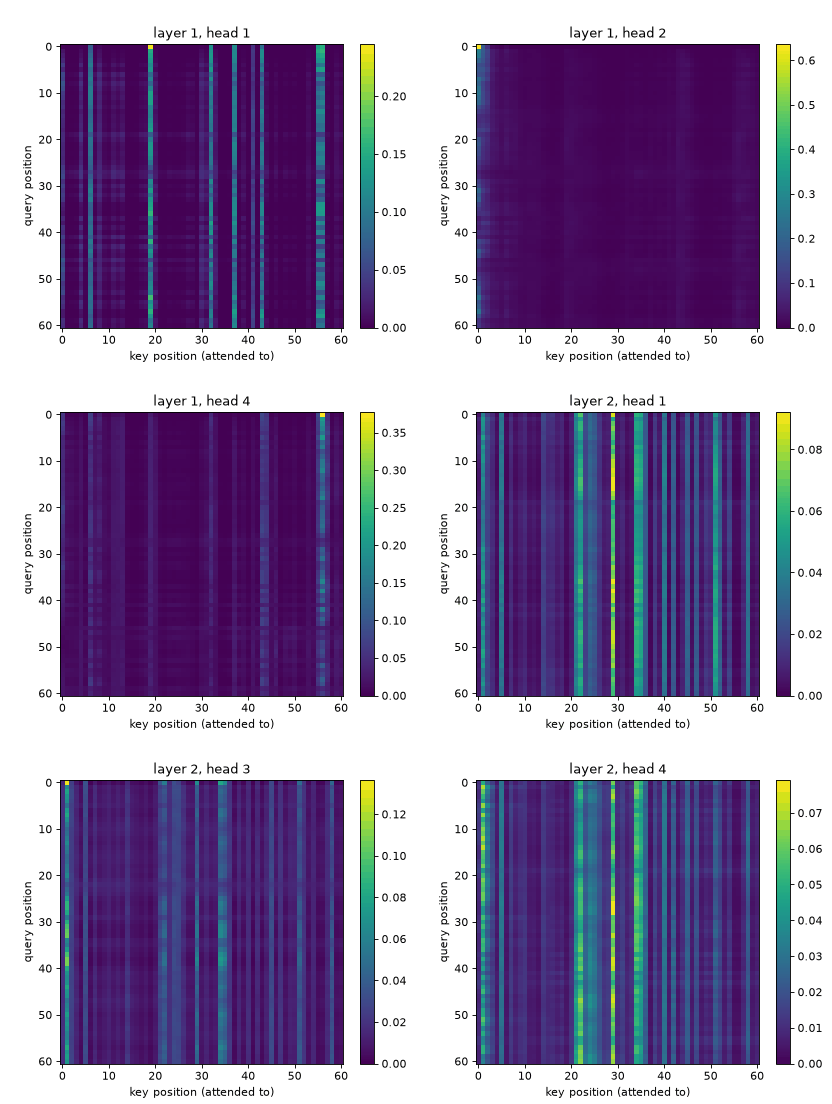 Every attention head of every layer, for one test sequence.
9. The Shortcut: nn.TransformerEncoder
Everything we built by hand exists in PyTorch already. Now that you know what is inside, use the built-in version — it is faster, better tested, and dispatches to fused kernels where available.
The one thing it does not give you easily is the attention weights, which is exactly why we wrote our own block first.
encoder_layer = nn.TransformerEncoderLayer(
    d_model=32, nhead=4, dim_feedforward=128,
    dropout=0.1, activation='gelu', batch_first=True, norm_first=True)
encoder = nn.TransformerEncoder(encoder_layer, num_layers=2)

sample = torch.randn(2, SEQ_LEN + 1, 32)
print('Built-in encoder output:', tuple(encoder(sample).shape))
print(f'Parameters: {sum(p.numel() for p in encoder.parameters()):,}')
print(f'Ours       : {sum(p.numel() for b in model.blocks for p in b.parameters()):,}')
print('\n`norm_first=True` is the pre-norm variant we used above.')
Built-in encoder output: (2, 61, 32)
Parameters: 25,408
Ours       : 25,408

`norm_first=True` is the pre-norm variant we used above.
C:\Users\injye\AppData\Local\Temp\ipykernel_26460\907610637.py:4: UserWarning: enable_nested_tensor is True, but self.use_nested_tensor is False because encoder_layer.norm_first was True
  encoder = nn.TransformerEncoder(encoder_layer, num_layers=2)
10. Experiment: Try Different Architectures and Hyperparameters
You can experiment with:
- Removing the positional encoding entirely — the task depends on which position holds the value, so accuracy should collapse to chance
- Raising
SEQ_LENto 300: attention should hold up where the LSTM from Lab 11 starts to struggle - Using
num_heads=1versusnum_heads=8at the samed_model - Replacing the CLS token with mean pooling over all positions, and comparing
- Passing a causal mask via
attn_maskand watching the attention maps become triangular - Swapping the sinusoidal encoding for a learned one:
nn.Embedding(max_len, d_model) - Timing a forward pass of the Transformer against the Lab 11 LSTM at
SEQ_LEN = 500, to feel the parallelism difference
Try modifying the model definition or training loop above and observe how the performance changes.
11. Conclusion
In this lab, you learned the mechanism behind modern sequence models. Attention replaces step-by-step recurrence with a direct, weighted lookup across all positions, which shortens every path to one hop and makes the whole sequence computable in parallel.
Key takeaways:
- Attention is a soft dictionary lookup: queries match keys, softmax turns matches into weights, values get averaged.
- The $\sqrt{d_k}$ scaling is not cosmetic — without it softmax saturates and gradients vanish.
- Multiple heads cost nothing extra and let the model attend in several ways at once.
- Attention is order-blind by construction, so position information must be added explicitly.
- A Transformer block is attention + feed-forward, each wrapped in a residual and a layer norm.
- The attention weights are inspectable, which makes these models far easier to debug than RNNs.
The next lab changes direction: instead of predicting labels, we train networks to generate data.