Lab 17: Deployment and Model Optimization¶

Every lab so far ended when the accuracy printed. In a real project that is roughly the halfway point. A model that only runs inside the notebook that trained it is not a product — it has to be saved reliably, loaded somewhere else, made fast enough, and wrapped in something another program can call.

This lab is about that second half.

We will cover the following topics:

• Saving and loading models without the traps
• Inference hygiene: eval(), inference_mode(), and batching
• TorchScript: freezing a model into a portable graph, and when tracing lies to you
• Exporting to ONNX for runtimes that have never heard of Python
• Quantization: smaller and faster, for a little accuracy
• Benchmarking honestly, and a deployment checklist

1. From Notebook to Something You Can Ship¶

Each stage trades flexibility for speed. The Python model is the easiest to change and the slowest to run; a quantised, compiled graph is the opposite. Most projects stop somewhere in the middle, and the right stopping point depends on where the model has to run — a server with a GPU, a phone, or a microcontroller.

Let's train something small first, so we have a real artefact to work with.

In [1]:

import torch
import torch.nn as nn
import torch.optim as optim
import numpy as np
import matplotlib.pyplot as plt
import os
import time
from torch.utils.data import DataLoader
from torchvision import datasets, transforms

torch.manual_seed(0)
device = torch.device('cuda' if torch.cuda.is_available() else 'cpu')
print('PyTorch version:', torch.__version__, '| device:', device)

tf = transforms.Compose([
    transforms.ToTensor(),
    transforms.Normalize((0.1307,), (0.3081,)),
])
train_set = datasets.MNIST(root='./data', train=True, download=True, transform=tf)
test_set = datasets.MNIST(root='./data', train=False, download=True, transform=tf)
train_loader = DataLoader(train_set, batch_size=128, shuffle=True)
test_loader = DataLoader(test_set, batch_size=512, shuffle=False)

import torch import torch.nn as nn import torch.optim as optim import numpy as np import matplotlib.pyplot as plt import os import time from torch.utils.data import DataLoader from torchvision import datasets, transforms torch.manual_seed(0) device = torch.device('cuda' if torch.cuda.is_available() else 'cpu') print('PyTorch version:', torch.__version__, '| device:', device) tf = transforms.Compose([ transforms.ToTensor(), transforms.Normalize((0.1307,), (0.3081,)), ]) train_set = datasets.MNIST(root='./data', train=True, download=True, transform=tf) test_set = datasets.MNIST(root='./data', train=False, download=True, transform=tf) train_loader = DataLoader(train_set, batch_size=128, shuffle=True) test_loader = DataLoader(test_set, batch_size=512, shuffle=False)

PyTorch version: 2.13.0+cpu | device: cpu

In [2]:

class DigitCNN(nn.Module):
    """The Lab 09 CNN, with a fat classifier head so quantization has something to work on."""
    def __init__(self, num_classes=10):
        super(DigitCNN, self).__init__()
        self.features = nn.Sequential(
            nn.Conv2d(1, 16, 3, padding=1), nn.ReLU(), nn.MaxPool2d(2),
            nn.Conv2d(16, 32, 3, padding=1), nn.ReLU(), nn.MaxPool2d(2),
        )
        self.classifier = nn.Sequential(
            nn.Flatten(),
            nn.Linear(32 * 7 * 7, 256), nn.ReLU(),
            nn.Linear(256, num_classes),
        )

    def forward(self, x):
        return self.classifier(self.features(x))

model = DigitCNN().to(device)
criterion = nn.CrossEntropyLoss()
optimizer = optim.Adam(model.parameters(), lr=1e-3)

for epoch in range(2):
    model.train()
    for images, labels in train_loader:
        images, labels = images.to(device), labels.to(device)
        optimizer.zero_grad()
        loss = criterion(model(images), labels)
        loss.backward()
        optimizer.step()
    print(f'Epoch {epoch + 1} done, last batch loss {loss.item():.4f}')

def accuracy(m, loader=test_loader, dev=None):
    if dev is None:
        params = list(m.parameters())
        dev = params[0].device if params else torch.device('cpu')
    m.eval()
    correct = total = 0
    with torch.inference_mode():
        for images, labels in loader:
            preds = m(images.to(dev)).argmax(1).cpu()
            correct += (preds == labels).sum().item()
            total += labels.size(0)
    return 100 * correct / total

baseline_acc = accuracy(model)
print(f'Test accuracy: {baseline_acc:.2f}%')

class DigitCNN(nn.Module): """The Lab 09 CNN, with a fat classifier head so quantization has something to work on.""" def __init__(self, num_classes=10): super(DigitCNN, self).__init__() self.features = nn.Sequential( nn.Conv2d(1, 16, 3, padding=1), nn.ReLU(), nn.MaxPool2d(2), nn.Conv2d(16, 32, 3, padding=1), nn.ReLU(), nn.MaxPool2d(2), ) self.classifier = nn.Sequential( nn.Flatten(), nn.Linear(32 * 7 * 7, 256), nn.ReLU(), nn.Linear(256, num_classes), ) def forward(self, x): return self.classifier(self.features(x)) model = DigitCNN().to(device) criterion = nn.CrossEntropyLoss() optimizer = optim.Adam(model.parameters(), lr=1e-3) for epoch in range(2): model.train() for images, labels in train_loader: images, labels = images.to(device), labels.to(device) optimizer.zero_grad() loss = criterion(model(images), labels) loss.backward() optimizer.step() print(f'Epoch {epoch + 1} done, last batch loss {loss.item():.4f}') def accuracy(m, loader=test_loader, dev=None): if dev is None: params = list(m.parameters()) dev = params[0].device if params else torch.device('cpu') m.eval() correct = total = 0 with torch.inference_mode(): for images, labels in loader: preds = m(images.to(dev)).argmax(1).cpu() correct += (preds == labels).sum().item() total += labels.size(0) return 100 * correct / total baseline_acc = accuracy(model) print(f'Test accuracy: {baseline_acc:.2f}%')

Epoch 1 done, last batch loss 0.0777

Epoch 2 done, last batch loss 0.0174

Test accuracy: 98.84%

2. Saving and Loading, Properly¶

Three ways to persist a model, in increasing order of how much you should trust them:

1. torch.save(model, path) — the whole object. Convenient, and a trap. Pickle stores a reference to your class, not its code, so loading requires the exact same module layout. Rename the file that defines DigitCNN and the checkpoint stops loading.

2. torch.save(model.state_dict(), path) — just the tensors. Portable and refactor-proof. You rebuild the architecture in code, then pour the weights in. This is the default choice.

3. A full checkpoint dict. The state_dict plus the optimizer state, the epoch, and anything else needed to resume training rather than only run inference.

In [3]:

os.makedirs('artifacts', exist_ok=True)

# The one you should normally use
torch.save(model.state_dict(), 'artifacts/model_weights.pt')

# A resumable training checkpoint
torch.save({
    'epoch': 2,
    'model_state': model.state_dict(),
    'optimizer_state': optimizer.state_dict(),
    'accuracy': baseline_acc,
    'classes': list(range(10)),
}, 'artifacts/checkpoint.pt')

for name in ['model_weights.pt', 'checkpoint.pt']:
    size = os.path.getsize(f'artifacts/{name}') / 1e6
    print(f'{name:22s} {size:6.2f} MB')
print('\nThe checkpoint is larger because Adam stores two moment tensors per parameter.')

os.makedirs('artifacts', exist_ok=True) # The one you should normally use torch.save(model.state_dict(), 'artifacts/model_weights.pt') # A resumable training checkpoint torch.save({ 'epoch': 2, 'model_state': model.state_dict(), 'optimizer_state': optimizer.state_dict(), 'accuracy': baseline_acc, 'classes': list(range(10)), }, 'artifacts/checkpoint.pt') for name in ['model_weights.pt', 'checkpoint.pt']: size = os.path.getsize(f'artifacts/{name}') / 1e6 print(f'{name:22s} {size:6.2f} MB') print('\nThe checkpoint is larger because Adam stores two moment tensors per parameter.')

model_weights.pt         1.64 MB
checkpoint.pt            4.92 MB

The checkpoint is larger because Adam stores two moment tensors per parameter.

In [4]:

# Loading for inference: rebuild, load, eval, move
loaded = DigitCNN()
state = torch.load('artifacts/model_weights.pt', map_location='cpu', weights_only=True)
loaded.load_state_dict(state)
loaded.eval()
loaded.to(device)

print(f'Reloaded accuracy: {accuracy(loaded):.2f}%')

# Resuming training instead
ckpt = torch.load('artifacts/checkpoint.pt', map_location='cpu', weights_only=True)
resumed = DigitCNN()
resumed.load_state_dict(ckpt['model_state'])
resumed_opt = optim.Adam(resumed.parameters())
resumed_opt.load_state_dict(ckpt['optimizer_state'])
print(f"Resuming from epoch {ckpt['epoch']} (saved accuracy {ckpt['accuracy']:.2f}%)")

# Loading for inference: rebuild, load, eval, move loaded = DigitCNN() state = torch.load('artifacts/model_weights.pt', map_location='cpu', weights_only=True) loaded.load_state_dict(state) loaded.eval() loaded.to(device) print(f'Reloaded accuracy: {accuracy(loaded):.2f}%') # Resuming training instead ckpt = torch.load('artifacts/checkpoint.pt', map_location='cpu', weights_only=True) resumed = DigitCNN() resumed.load_state_dict(ckpt['model_state']) resumed_opt = optim.Adam(resumed.parameters()) resumed_opt.load_state_dict(ckpt['optimizer_state']) print(f"Resuming from epoch {ckpt['epoch']} (saved accuracy {ckpt['accuracy']:.2f}%)")

Reloaded accuracy: 98.84%
Resuming from epoch 2 (saved accuracy 98.84%)

Three details that cause real incidents:

• map_location='cpu'. A checkpoint saved from a GPU remembers that, and loading it on a CPU-only machine fails outright. Always load to CPU, then .to(device).
• weights_only=True. torch.load unpickles, and unpickling arbitrary files can execute arbitrary code. Never load a checkpoint you did not produce without it. Recent PyTorch versions default to True for exactly this reason.
• model.eval() before serving. Dropout and batch norm behave differently in training mode. Forgetting this gives you a model that is quietly, randomly worse — and it will not raise an error.

3. Inference Hygiene¶

Two easy wins before any clever optimization.

torch.inference_mode() turns off autograd bookkeeping entirely. It is a stricter, faster successor to torch.no_grad(): no graph, no version counters. Use it for every forward pass you are not going to backpropagate through.

Batching. Per-call overhead — the Python call, the kernel launch, the memory transfer — is roughly fixed. Amortising it across 64 inputs instead of one is usually the single biggest speedup available, and it costs nothing but latency on the first item.

In [5]:

def benchmark(fn, x, runs=50, warmup=5):
    """Median wall-clock time per call, in milliseconds."""
    for _ in range(warmup):          # warm up caches, lazy init, autotuning
        fn(x)
    if device.type == 'cuda':
        torch.cuda.synchronize()
    times = []
    for _ in range(runs):
        t0 = time.perf_counter()
        fn(x)
        if device.type == 'cuda':
            torch.cuda.synchronize()
        times.append((time.perf_counter() - t0) * 1000)
    return float(np.median(times))

model.eval()

def with_grad(x):
    return model(x)

def without_grad(x):
    with torch.inference_mode():
        return model(x)

sample = torch.randn(32, 1, 28, 28, device=device)
print(f'autograd on          : {benchmark(with_grad, sample):.2f} ms per batch of 32')
print(f'inference_mode       : {benchmark(without_grad, sample):.2f} ms per batch of 32')

def benchmark(fn, x, runs=50, warmup=5): """Median wall-clock time per call, in milliseconds.""" for _ in range(warmup): # warm up caches, lazy init, autotuning fn(x) if device.type == 'cuda': torch.cuda.synchronize() times = [] for _ in range(runs): t0 = time.perf_counter() fn(x) if device.type == 'cuda': torch.cuda.synchronize() times.append((time.perf_counter() - t0) * 1000) return float(np.median(times)) model.eval() def with_grad(x): return model(x) def without_grad(x): with torch.inference_mode(): return model(x) sample = torch.randn(32, 1, 28, 28, device=device) print(f'autograd on : {benchmark(with_grad, sample):.2f} ms per batch of 32') print(f'inference_mode : {benchmark(without_grad, sample):.2f} ms per batch of 32')

autograd on          : 8.63 ms per batch of 32

inference_mode       : 8.20 ms per batch of 32

In [6]:

batch_sizes = [1, 2, 4, 8, 16, 32, 64, 128, 256]
per_item, throughput = [], []

for bs in batch_sizes:
    x = torch.randn(bs, 1, 28, 28, device=device)
    ms = benchmark(without_grad, x, runs=30)
    per_item.append(ms / bs)
    throughput.append(bs / (ms / 1000))

fig, (ax1, ax2) = plt.subplots(1, 2, figsize=(11, 4))
ax1.plot(batch_sizes, per_item, marker='o')
ax1.set_xscale('log', base=2); ax1.set_yscale('log')
ax1.set_xlabel('batch size'); ax1.set_ylabel('ms per image')
ax1.set_title('Cost per image collapses with batching')
ax1.grid(alpha=0.3, which='both')

ax2.plot(batch_sizes, throughput, marker='o', color='#55A868')
ax2.set_xscale('log', base=2)
ax2.set_xlabel('batch size'); ax2.set_ylabel('images per second')
ax2.set_title('Throughput')
ax2.grid(alpha=0.3)
plt.tight_layout()
plt.show()

print(f'Batch of 1  : {per_item[0]:.3f} ms per image')
print(f'Batch of 256: {per_item[-1]:.3f} ms per image  '
      f'({per_item[0] / per_item[-1]:.0f}x cheaper per image)')

batch_sizes = [1, 2, 4, 8, 16, 32, 64, 128, 256] per_item, throughput = [], [] for bs in batch_sizes: x = torch.randn(bs, 1, 28, 28, device=device) ms = benchmark(without_grad, x, runs=30) per_item.append(ms / bs) throughput.append(bs / (ms / 1000)) fig, (ax1, ax2) = plt.subplots(1, 2, figsize=(11, 4)) ax1.plot(batch_sizes, per_item, marker='o') ax1.set_xscale('log', base=2); ax1.set_yscale('log') ax1.set_xlabel('batch size'); ax1.set_ylabel('ms per image') ax1.set_title('Cost per image collapses with batching') ax1.grid(alpha=0.3, which='both') ax2.plot(batch_sizes, throughput, marker='o', color='#55A868') ax2.set_xscale('log', base=2) ax2.set_xlabel('batch size'); ax2.set_ylabel('images per second') ax2.set_title('Throughput') ax2.grid(alpha=0.3) plt.tight_layout() plt.show() print(f'Batch of 1 : {per_item[0]:.3f} ms per image') print(f'Batch of 256: {per_item[-1]:.3f} ms per image ' f'({per_item[0] / per_item[-1]:.0f}x cheaper per image)')

Batch of 1  : 0.720 ms per image
Batch of 256: 0.188 ms per image  (4x cheaper per image)

4. TorchScript: Leaving Python Behind¶

A PyTorch model is Python code, and running it needs a Python interpreter. TorchScript compiles it into a serialised graph that the C++ runtime can execute — no Python, no source files, one self-contained artefact.

There are two ways in, and the difference matters:

• torch.jit.trace runs your model on an example input and records the operations that actually executed. Fast, works on almost anything — and it silently discards control flow. Whichever branch the example took is the branch that gets baked in, forever.
• torch.jit.script compiles the source directly, keeping ifs and loops. Stricter about what Python it accepts, but correct.

Use script when the forward pass has data-dependent behaviour. Use trace when it does not.

In [7]:

cpu_model = DigitCNN()
cpu_model.load_state_dict(torch.load('artifacts/model_weights.pt',
                                     map_location='cpu', weights_only=True))
cpu_model.eval()

example = torch.randn(1, 1, 28, 28)

traced = torch.jit.trace(cpu_model, example)
scripted = torch.jit.script(cpu_model)

torch.jit.save(traced, 'artifacts/model_traced.pt')
torch.jit.save(scripted, 'artifacts/model_scripted.pt')

# The saved file needs no model class at all to load
reloaded = torch.jit.load('artifacts/model_traced.pt')
with torch.inference_mode():
    same = torch.allclose(reloaded(example), cpu_model(example), atol=1e-5)
print('TorchScript output matches the original:', same)
for name in ['model_weights.pt', 'model_traced.pt', 'model_scripted.pt']:
    print(f'  {name:22s} {os.path.getsize("artifacts/" + name) / 1e6:5.2f} MB')

cpu_model = DigitCNN() cpu_model.load_state_dict(torch.load('artifacts/model_weights.pt', map_location='cpu', weights_only=True)) cpu_model.eval() example = torch.randn(1, 1, 28, 28) traced = torch.jit.trace(cpu_model, example) scripted = torch.jit.script(cpu_model) torch.jit.save(traced, 'artifacts/model_traced.pt') torch.jit.save(scripted, 'artifacts/model_scripted.pt') # The saved file needs no model class at all to load reloaded = torch.jit.load('artifacts/model_traced.pt') with torch.inference_mode(): same = torch.allclose(reloaded(example), cpu_model(example), atol=1e-5) print('TorchScript output matches the original:', same) for name in ['model_weights.pt', 'model_traced.pt', 'model_scripted.pt']: print(f' {name:22s} {os.path.getsize("artifacts/" + name) / 1e6:5.2f} MB')

TorchScript output matches the original: True
  model_weights.pt        1.64 MB
  model_traced.pt         1.66 MB
  model_scripted.pt       1.66 MB

Tracing, caught in the act¶

This is worth seeing rather than taking on faith. Here is a model whose behaviour depends on its input; we trace it with one kind of input and then feed it another.

In [8]:

class ConditionalModel(nn.Module):
    def forward(self, x):
        if x.sum() > 0:
            return x * 10          # the "positive" branch
        return x * -1              # the "negative" branch

cond = ConditionalModel()
positive = torch.ones(3)
negative = -torch.ones(3)

traced_cond = torch.jit.trace(cond, positive)     # traced through the positive branch only
scripted_cond = torch.jit.script(cond)

print('           eager      traced     scripted')
for name, inp in [('positive', positive), ('negative', negative)]:
    print(f'{name:9s}  {cond(inp).tolist()}  {traced_cond(inp).tolist()}  '
          f'{scripted_cond(inp).tolist()}')
print('\nThe traced model returns the wrong answer for negative input, with no error and')
print('no warning at inference time. Only the trace-time warning above hints at it.')

class ConditionalModel(nn.Module): def forward(self, x): if x.sum() > 0: return x * 10 # the "positive" branch return x * -1 # the "negative" branch cond = ConditionalModel() positive = torch.ones(3) negative = -torch.ones(3) traced_cond = torch.jit.trace(cond, positive) # traced through the positive branch only scripted_cond = torch.jit.script(cond) print(' eager traced scripted') for name, inp in [('positive', positive), ('negative', negative)]: print(f'{name:9s} {cond(inp).tolist()} {traced_cond(inp).tolist()} ' f'{scripted_cond(inp).tolist()}') print('\nThe traced model returns the wrong answer for negative input, with no error and') print('no warning at inference time. Only the trace-time warning above hints at it.')

           eager      traced     scripted
positive   [10.0, 10.0, 10.0]  [10.0, 10.0, 10.0]  [10.0, 10.0, 10.0]
negative   [1.0, 1.0, 1.0]  [-10.0, -10.0, -10.0]  [1.0, 1.0, 1.0]

The traced model returns the wrong answer for negative input, with no error and
no warning at inference time. Only the trace-time warning above hints at it.

C:\Users\injye\AppData\Local\Temp\ipykernel_6084\2754063520.py:3: TracerWarning: Converting a tensor to a Python boolean might cause the trace to be incorrect. We can't record the data flow of Python values, so this value will be treated as a constant in the future. This means that the trace might not generalize to other inputs!
  if x.sum() > 0:

5. ONNX: Leaving PyTorch Behind¶

ONNX is an interchange format. Export once, and the model runs under ONNX Runtime, TensorRT, CoreML, or a browser via WebAssembly — none of which need PyTorch installed.

The important argument is dynamic_shapes. Without it, the exported graph is locked to the exact batch size of your example input, and serving a batch of 7 to a model exported with batch 1 fails.

Two notes on the API, because it changed recently:

• Modern PyTorch exports through torch.export (the "dynamo" path) by default. It needs the onnxscript package installed: pip install onnxscript.
• The older dynamic_axes={'input': {0: 'batch'}} argument still works through a compatibility shim, but it is deprecated. The current form declares a symbolic dimension with torch.export.Dim and keys the dict by the argument names of forward — our forward(self, x) means the key is x, not the ONNX input name.

In [9]:

onnx_path = 'artifacts/model.onnx'
batch_dim = torch.export.Dim('batch')      # a dimension that is allowed to vary

torch.onnx.export(
    cpu_model,
    (example,),
    onnx_path,
    input_names=['input'],
    output_names=['logits'],
    dynamic_shapes={'x': {0: batch_dim}},   # 'x' is the parameter name in forward()
    opset_version=17,
    dynamo=True,
)
print(f'Exported {onnx_path} ({os.path.getsize(onnx_path) / 1e6:.2f} MB)')

# Verifying the export needs onnxruntime, which is an optional extra install
try:
    import onnxruntime as ort
    session = ort.InferenceSession(onnx_path, providers=['CPUExecutionProvider'])
    print('declared input shape:', session.get_inputs()[0].shape,
          "  <- 'batch' stayed symbolic\n")
    for batch in [1, 7, 32]:
        x = torch.randn(batch, 1, 28, 28)
        onnx_out = session.run(None, {'input': x.numpy()})[0]
        with torch.inference_mode():
            torch_out = cpu_model(x).numpy()
        print(f'  batch {batch:3d}: max difference '
              f'{np.abs(onnx_out - torch_out).max():.2e}')
except ImportError:
    print('onnxruntime is not installed - skipping verification.')
    print('Install it with:  pip install onnxruntime')

onnx_path = 'artifacts/model.onnx' batch_dim = torch.export.Dim('batch') # a dimension that is allowed to vary torch.onnx.export( cpu_model, (example,), onnx_path, input_names=['input'], output_names=['logits'], dynamic_shapes={'x': {0: batch_dim}}, # 'x' is the parameter name in forward() opset_version=17, dynamo=True, ) print(f'Exported {onnx_path} ({os.path.getsize(onnx_path) / 1e6:.2f} MB)') # Verifying the export needs onnxruntime, which is an optional extra install try: import onnxruntime as ort session = ort.InferenceSession(onnx_path, providers=['CPUExecutionProvider']) print('declared input shape:', session.get_inputs()[0].shape, " <- 'batch' stayed symbolic\n") for batch in [1, 7, 32]: x = torch.randn(batch, 1, 28, 28) onnx_out = session.run(None, {'input': x.numpy()})[0] with torch.inference_mode(): torch_out = cpu_model(x).numpy() print(f' batch {batch:3d}: max difference ' f'{np.abs(onnx_out - torch_out).max():.2e}') except ImportError: print('onnxruntime is not installed - skipping verification.') print('Install it with: pip install onnxruntime')

W0814 14:26:09.059000 6084 site-packages\torch\onnx\_internal\exporter\_compat.py:133] Setting ONNX exporter to use operator set version 18 because the requested opset_version 17 is a lower version than we have implementations for. Automatic version conversion will be performed, which may not be successful at converting to the requested version. If version conversion is unsuccessful, the opset version of the exported model will be kept at 18. Please consider setting opset_version >=18 to leverage latest ONNX features

[torch.onnx] Obtain model graph for `DigitCNN([...]` with `torch.export.export(..., strict=False)`...

[torch.onnx] Obtain model graph for `DigitCNN([...]` with `torch.export.export(..., strict=False)`... ✅
[torch.onnx] Run decompositions...

C:\Users\injye\.conda\envs\envNeural\Lib\copyreg.py:99: FutureWarning: `isinstance(treespec, LeafSpec)` is deprecated, use `isinstance(treespec, TreeSpec) and treespec.is_leaf()` instead.
  return cls.__new__(cls, *args)
The model version conversion is not supported by the onnxscript version converter and fallback is enabled. The model will be converted using the onnx C API (target version: 17).

[torch.onnx] Run decompositions... ✅
[torch.onnx] Translate the graph into ONNX...
[torch.onnx] Translate the graph into ONNX... ✅
[torch.onnx] Optimize the ONNX graph...

[torch.onnx] Optimize the ONNX graph... ✅
Exported artifacts/model.onnx (0.00 MB)

declared input shape: ['batch', 1, 28, 28]   <- 'batch' stayed symbolic

  batch   1: max difference 1.91e-06

  batch   7: max difference 1.19e-06

  batch  32: max difference 1.43e-06

6. Quantization¶

Weights are stored as 32-bit floats, and mostly they do not need to be. Quantization stores them as 8-bit integers instead: a quarter of the memory, and integer arithmetic that is faster on most CPUs.

Two flavours:

• Dynamic quantization quantises weights ahead of time and activations on the fly. One line of code, no calibration data, works well for Linear and recurrent layers. This is the one to try first.
• Static quantization also quantises activations ahead of time, using a calibration pass over sample data. Faster still, more work, and usually better for convolutional networks.

Our model's two Linear layers hold most of its parameters, so dynamic quantization has plenty to bite on. Note that quantized models run on CPU only.

In [10]:

from torch.ao.quantization import quantize_dynamic

quantized = quantize_dynamic(cpu_model, {nn.Linear}, dtype=torch.qint8)
torch.save(quantized.state_dict(), 'artifacts/model_quantized.pt')

fp32_size = os.path.getsize('artifacts/model_weights.pt') / 1e6
int8_size = os.path.getsize('artifacts/model_quantized.pt') / 1e6
print(f'float32 weights: {fp32_size:.2f} MB')
print(f'int8 weights   : {int8_size:.2f} MB  ({fp32_size / int8_size:.1f}x smaller)')

quant_acc = accuracy(quantized, dev=torch.device('cpu'))
fp32_cpu_acc = accuracy(cpu_model, dev=torch.device('cpu'))
print(f'\nfloat32 accuracy: {fp32_cpu_acc:.2f}%')
print(f'int8 accuracy   : {quant_acc:.2f}%  ({quant_acc - fp32_cpu_acc:+.2f} points)')

from torch.ao.quantization import quantize_dynamic quantized = quantize_dynamic(cpu_model, {nn.Linear}, dtype=torch.qint8) torch.save(quantized.state_dict(), 'artifacts/model_quantized.pt') fp32_size = os.path.getsize('artifacts/model_weights.pt') / 1e6 int8_size = os.path.getsize('artifacts/model_quantized.pt') / 1e6 print(f'float32 weights: {fp32_size:.2f} MB') print(f'int8 weights : {int8_size:.2f} MB ({fp32_size / int8_size:.1f}x smaller)') quant_acc = accuracy(quantized, dev=torch.device('cpu')) fp32_cpu_acc = accuracy(cpu_model, dev=torch.device('cpu')) print(f'\nfloat32 accuracy: {fp32_cpu_acc:.2f}%') print(f'int8 accuracy : {quant_acc:.2f}% ({quant_acc - fp32_cpu_acc:+.2f} points)')

C:\Users\injye\AppData\Local\Temp\ipykernel_6084\4180530815.py:3: DeprecationWarning: torch.ao.quantization is deprecated and will be removed in 2.10. 
For migrations of users: 
1. Eager mode quantization (torch.ao.quantization.quantize, torch.ao.quantization.quantize_dynamic), please migrate to use torchao eager mode quantize_ API instead 
2. FX graph mode quantization (torch.ao.quantization.quantize_fx.prepare_fx,torch.ao.quantization.quantize_fx.convert_fx, please migrate to use torchao pt2e quantization API instead (prepare_pt2e, convert_pt2e) 
3. pt2e quantization has been migrated to torchao (https://github.com/pytorch/ao/tree/main/torchao/quantization/pt2e) 
see https://github.com/pytorch/ao/issues/2259 for more details
  quantized = quantize_dynamic(cpu_model, {nn.Linear}, dtype=torch.qint8)
C:\Users\injye\.conda\envs\envNeural\Lib\site-packages\torch\ao\nn\quantized\modules\utils.py:72: UserWarning: torch.quantize_per_tensor, torch.quantize_per_channel and other quantized tensor creation functions that produce tensors with dtype torch.quint8, torch.qint8, and torch.qint32 are deprecated and will be removed in a future PyTorch release. Please see https://github.com/pytorch/pytorch/issues/184982 for more information. (Triggered internally at C:\actions-runner\_work\pytorch\pytorch\aten\src\ATen\quantized\Quantizer.cpp:116.)
  qweight = torch.quantize_per_tensor(

float32 weights: 1.64 MB
int8 weights   : 0.43 MB  (3.8x smaller)

float32 accuracy: 98.84%
int8 accuracy   : 98.83%  (-0.01 points)

In [11]:

# Latency comparison, all on CPU so the numbers are comparable
cpu_batch = torch.randn(32, 1, 28, 28)

def run_cpu(m):
    def inner(x):
        with torch.inference_mode():
            return m(x)
    return inner

variants = {
    'eager fp32': run_cpu(cpu_model),
    'traced fp32': run_cpu(torch.jit.load('artifacts/model_traced.pt')),
    'dynamic int8': run_cpu(quantized),
}

latency = {name: benchmark(fn, cpu_batch, runs=40) for name, fn in variants.items()}
for name, ms in latency.items():
    print(f'{name:14s} {ms:6.2f} ms per batch of 32')

fig, ax = plt.subplots(figsize=(7, 3.6))
names = list(latency)
values = [latency[n] for n in names]
ax.barh(names, values, color=['#4C72B0', '#8172B3', '#55A868'])
for i, v in enumerate(values):
    ax.text(v + max(values) * 0.02, i, f'{v:.2f} ms', va='center', fontsize=9)
ax.set_xlim(0, max(values) * 1.25)
ax.set_xlabel('milliseconds per batch of 32 (CPU, lower is better)')
ax.set_title('What each optimization bought')
plt.tight_layout()
plt.show()
print('Results vary a lot by CPU. Measure on the hardware you will actually deploy to.')

# Latency comparison, all on CPU so the numbers are comparable cpu_batch = torch.randn(32, 1, 28, 28) def run_cpu(m): def inner(x): with torch.inference_mode(): return m(x) return inner variants = { 'eager fp32': run_cpu(cpu_model), 'traced fp32': run_cpu(torch.jit.load('artifacts/model_traced.pt')), 'dynamic int8': run_cpu(quantized), } latency = {name: benchmark(fn, cpu_batch, runs=40) for name, fn in variants.items()} for name, ms in latency.items(): print(f'{name:14s} {ms:6.2f} ms per batch of 32') fig, ax = plt.subplots(figsize=(7, 3.6)) names = list(latency) values = [latency[n] for n in names] ax.barh(names, values, color=['#4C72B0', '#8172B3', '#55A868']) for i, v in enumerate(values): ax.text(v + max(values) * 0.02, i, f'{v:.2f} ms', va='center', fontsize=9) ax.set_xlim(0, max(values) * 1.25) ax.set_xlabel('milliseconds per batch of 32 (CPU, lower is better)') ax.set_title('What each optimization bought') plt.tight_layout() plt.show() print('Results vary a lot by CPU. Measure on the hardware you will actually deploy to.')

eager fp32      16.35 ms per batch of 32
traced fp32      8.93 ms per batch of 32
dynamic int8     7.73 ms per batch of 32

Results vary a lot by CPU. Measure on the hardware you will actually deploy to.

Other levers, in rough order of effort:

• torch.compile(model) — one line, and often a solid speedup on recent PyTorch. It compiles the graph with a JIT backend; the first call is slow while it warms up. Support varies by platform.
• Half precision (model.half() on CUDA, or torch.autocast) — roughly halves memory and is much faster on tensor-core GPUs.
• Static quantization with a calibration pass, for convolutional models.
• Pruning (torch.nn.utils.prune) — zeroing small weights. Real gains need sparse kernels or structured pruning.
• Knowledge distillation — train a small model to imitate a large one's outputs. Often the biggest win of all, and the most work.

7. A Serving Interface¶

The last step is to hide all of the above behind something another program can call. A predictor class should own exactly three responsibilities: load the artefact once, apply the same preprocessing used in training, and return a decision.

That middle one is where deployed models usually go wrong. If training normalised with mean 0.1307 and the server does not, the model will still return confident answers — just wrong ones. Keep the preprocessing next to the weights.

In [12]:

class DigitPredictor:
    """Everything needed to turn an image into a prediction, and nothing else."""

    MEAN, STD = 0.1307, 0.3081     # must match training

    def __init__(self, script_path, device='cpu'):
        self.device = torch.device(device)
        self.model = torch.jit.load(script_path, map_location=self.device)
        self.model.eval()

    def preprocess(self, images):
        """images: (N, 28, 28) float tensor in [0, 1], or a single (28, 28)."""
        if images.dim() == 2:
            images = images.unsqueeze(0)
        x = images.unsqueeze(1).float()               # (N, 1, 28, 28)
        return ((x - self.MEAN) / self.STD).to(self.device)

    @torch.inference_mode()
    def predict(self, images):
        logits = self.model(self.preprocess(images))
        probs = torch.softmax(logits, dim=1)
        confidence, label = probs.max(dim=1)
        return label.cpu().numpy(), confidence.cpu().numpy()

predictor = DigitPredictor('artifacts/model_traced.pt')

raw = datasets.MNIST(root='./data', train=False, download=True,
                     transform=transforms.ToTensor())
batch = torch.stack([raw[i][0][0] for i in range(8)])
truth = [raw[i][1] for i in range(8)]

labels, confs = predictor.predict(batch)
fig, axes = plt.subplots(1, 8, figsize=(11, 1.9))
for ax, img, pred, conf, true in zip(axes, batch, labels, confs, truth):
    ax.imshow(img, cmap='gray'); ax.axis('off')
    ax.set_title(f'{pred} ({conf:.0%})', fontsize=9,
                 color='black' if pred == true else 'red')
plt.tight_layout()
plt.show()

class DigitPredictor: """Everything needed to turn an image into a prediction, and nothing else.""" MEAN, STD = 0.1307, 0.3081 # must match training def __init__(self, script_path, device='cpu'): self.device = torch.device(device) self.model = torch.jit.load(script_path, map_location=self.device) self.model.eval() def preprocess(self, images): """images: (N, 28, 28) float tensor in [0, 1], or a single (28, 28).""" if images.dim() == 2: images = images.unsqueeze(0) x = images.unsqueeze(1).float() # (N, 1, 28, 28) return ((x - self.MEAN) / self.STD).to(self.device) @torch.inference_mode() def predict(self, images): logits = self.model(self.preprocess(images)) probs = torch.softmax(logits, dim=1) confidence, label = probs.max(dim=1) return label.cpu().numpy(), confidence.cpu().numpy() predictor = DigitPredictor('artifacts/model_traced.pt') raw = datasets.MNIST(root='./data', train=False, download=True, transform=transforms.ToTensor()) batch = torch.stack([raw[i][0][0] for i in range(8)]) truth = [raw[i][1] for i in range(8)] labels, confs = predictor.predict(batch) fig, axes = plt.subplots(1, 8, figsize=(11, 1.9)) for ax, img, pred, conf, true in zip(axes, batch, labels, confs, truth): ax.imshow(img, cmap='gray'); ax.axis('off') ax.set_title(f'{pred} ({conf:.0%})', fontsize=9, color='black' if pred == true else 'red') plt.tight_layout() plt.show()

Watching it serve¶

A quick simulation of the thing running: images arrive one at a time, the predictor answers, and we track latency as it goes.

In [13]:

from matplotlib import animation
import os

os.makedirs('Misc', exist_ok=True)

def save_animation(ani, filename, fps=8, dpi=80):
    """Render an animation to a GIF under Misc/ and report where it went."""
    path = os.path.join('Misc', filename)
    ani.save(path, writer='pillow', fps=fps, dpi=dpi)
    print(f'saved {path}  ({os.path.getsize(path) / 1e6:.1f} MB)')
    return path

stream = torch.stack([raw[i][0][0] for i in range(40)])
stream_truth = [raw[i][1] for i in range(40)]

results = []
for i in range(len(stream)):
    t0 = time.perf_counter()
    label, conf = predictor.predict(stream[i])
    results.append((int(label[0]), float(conf[0]), (time.perf_counter() - t0) * 1000))

fig, (ax_img, ax_lat) = plt.subplots(1, 2, figsize=(9, 3.4),
                                     gridspec_kw={'width_ratios': [1, 1.7]})
im = ax_img.imshow(stream[0], cmap='gray', vmin=0, vmax=1)
ax_img.axis('off')

lat = [r[2] for r in results]
line, = ax_lat.plot([], [], color='#4C72B0', marker='.')
ax_lat.set_xlim(0, len(stream) - 1)
ax_lat.set_ylim(0, max(lat) * 1.2)
ax_lat.set_xlabel('request'); ax_lat.set_ylabel('latency (ms)')
ax_lat.grid(alpha=0.3)

def update(k):
    pred, conf, ms = results[k]
    im.set_data(stream[k])
    ok = pred == stream_truth[k]
    ax_img.set_title(f'predicted {pred}  ({conf:.0%})', fontsize=10,
                     color='#55A868' if ok else '#C44E52')
    line.set_data(range(k + 1), lat[:k + 1])
    ax_lat.set_title(f'request {k + 1}: {ms:.2f} ms', fontsize=10)
    return im, line

ani = animation.FuncAnimation(fig, update, frames=len(stream), interval=200, blit=False)
plt.close(fig)
save_animation(ani, 'lab17_serving.gif', fps=5)

from matplotlib import animation import os os.makedirs('Misc', exist_ok=True) def save_animation(ani, filename, fps=8, dpi=80): """Render an animation to a GIF under Misc/ and report where it went.""" path = os.path.join('Misc', filename) ani.save(path, writer='pillow', fps=fps, dpi=dpi) print(f'saved {path} ({os.path.getsize(path) / 1e6:.1f} MB)') return path stream = torch.stack([raw[i][0][0] for i in range(40)]) stream_truth = [raw[i][1] for i in range(40)] results = [] for i in range(len(stream)): t0 = time.perf_counter() label, conf = predictor.predict(stream[i]) results.append((int(label[0]), float(conf[0]), (time.perf_counter() - t0) * 1000)) fig, (ax_img, ax_lat) = plt.subplots(1, 2, figsize=(9, 3.4), gridspec_kw={'width_ratios': [1, 1.7]}) im = ax_img.imshow(stream[0], cmap='gray', vmin=0, vmax=1) ax_img.axis('off') lat = [r[2] for r in results] line, = ax_lat.plot([], [], color='#4C72B0', marker='.') ax_lat.set_xlim(0, len(stream) - 1) ax_lat.set_ylim(0, max(lat) * 1.2) ax_lat.set_xlabel('request'); ax_lat.set_ylabel('latency (ms)') ax_lat.grid(alpha=0.3) def update(k): pred, conf, ms = results[k] im.set_data(stream[k]) ok = pred == stream_truth[k] ax_img.set_title(f'predicted {pred} ({conf:.0%})', fontsize=10, color='#55A868' if ok else '#C44E52') line.set_data(range(k + 1), lat[:k + 1]) ax_lat.set_title(f'request {k + 1}: {ms:.2f} ms', fontsize=10) return im, line ani = animation.FuncAnimation(fig, update, frames=len(stream), interval=200, blit=False) plt.close(fig) save_animation(ani, 'lab17_serving.gif', fps=5)

saved Misc\lab17_serving.gif  (0.3 MB)

Out[13]:

'Misc\\lab17_serving.gif'

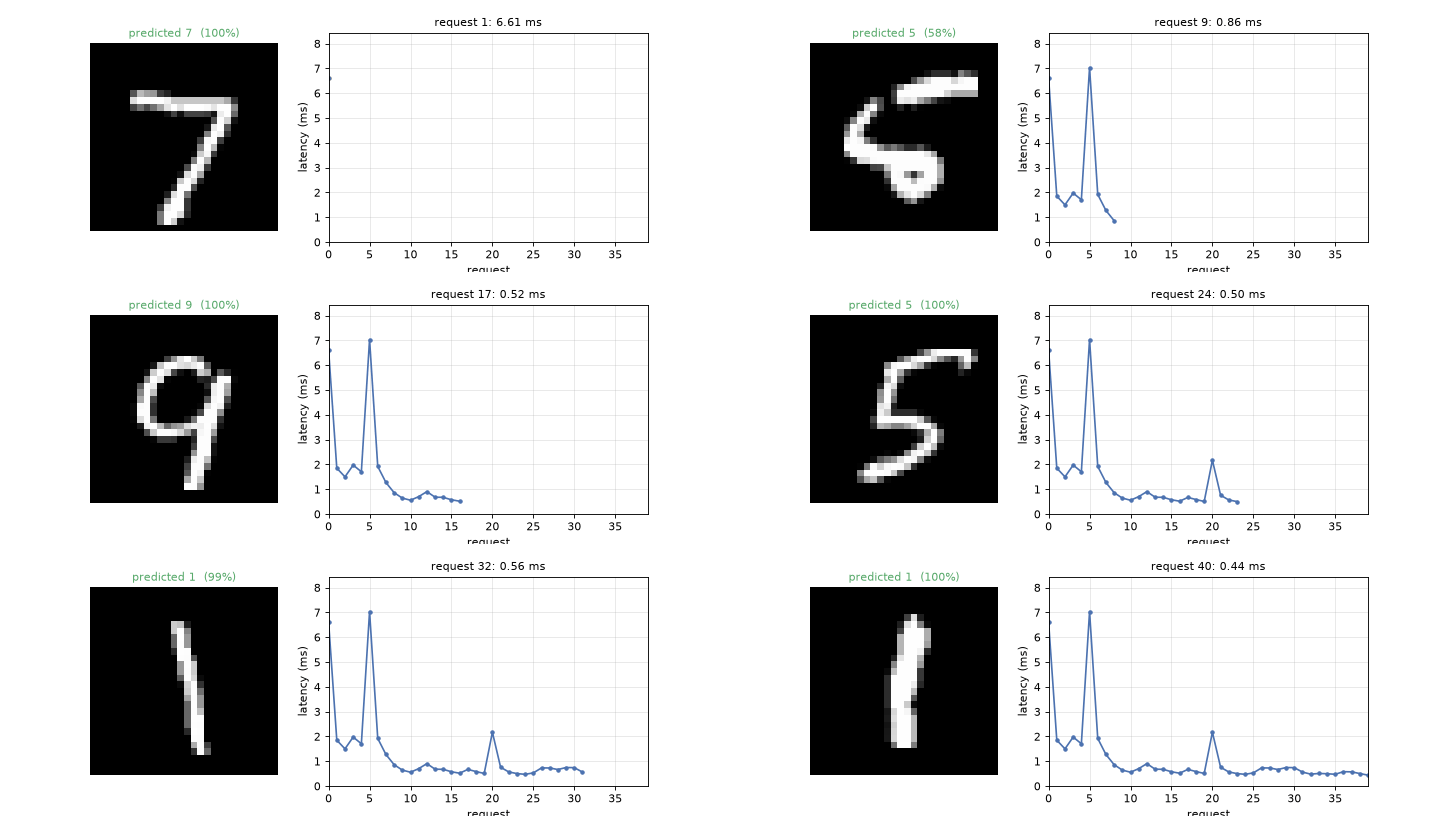The predictor answering one request at a time, with per-request latency.

Wrapping it in a web service¶

The predictor above is already the hard part. Turning it into an HTTP endpoint is a dozen lines — shown here rather than run, since a notebook is not a server:

# app.py  -  run with:  uvicorn app:app
from fastapi import FastAPI
from pydantic import BaseModel
import torch

app = FastAPI()
predictor = DigitPredictor('artifacts/model_traced.pt')   # loaded once, at startup

class Request(BaseModel):
    pixels: list[list[float]]        # a 28x28 grid in [0, 1]

@app.post('/predict')
def predict(req: Request):
    image = torch.tensor(req.pixels)
    label, confidence = predictor.predict(image)
    return {'digit': int(label[0]), 'confidence': float(confidence[0])}

Load the model once at startup, never per request — loading is far more expensive than inference. Beyond that, production serving is mostly ordinary engineering: request batching, health checks, monitoring the input distribution for drift, and a way to roll back to the previous model.

8. A Deployment Checklist¶

Before a model goes anywhere:

• Weights saved as a state_dict, with the architecture defined in version-controlled code
• Preprocessing constants stored with the model, not retyped at the call site
• model.eval() called, and verified — compare a known input's output before and after
• Loading uses map_location and weights_only=True
• Accuracy re-measured after every optimization step, not assumed
• Latency measured on the target hardware, with a warmup, at the real batch size
• Behaviour checked on bad input: wrong shape, wrong dtype, all zeros, an empty batch
• The model version recorded in the response, so a bad prediction can be traced to a build

9. Experiment: Try Different Optimizations¶

You can experiment with:

• Running torch.compile(cpu_model) and re-benchmarking (expect a slow first call; support varies by platform)
• Applying static quantization with a calibration pass, and comparing against the dynamic result
• Exporting to ONNX and benchmarking under onnxruntime against eager PyTorch
• Pruning 50% of the weights with torch.nn.utils.prune.l1_unstructured and measuring accuracy, size and speed separately — the three do not move together
• Distilling DigitCNN into a much smaller student network trained on its softened outputs
• Measuring how much of the "inference time" is actually preprocessing rather than the model
• Deliberately breaking the preprocessing in DigitPredictor (drop the normalisation) to see how quietly wrong a deployed model can be

Try modifying the code above and observe how the numbers change.

10. Conclusion¶

In this lab, you took a trained model out of the notebook: saved it properly, compiled it to TorchScript, exported it to ONNX, quantised it to int8, benchmarked each step, and wrapped the result in a serving interface.

Key takeaways:

• Save the state_dict; keep the architecture in code.
• map_location, weights_only=True and model.eval() are three lines that prevent three classes of incident.
• Batching and inference_mode() are free speedups; take them before anything clever.
• torch.jit.trace discards control flow silently — use script when the forward pass branches.
• Quantization gives about 4x smaller and meaningfully faster for a fraction of a point of accuracy.
• Preprocessing must match training exactly, or the model fails silently rather than loudly.
• Measure everything on the hardware you will deploy to, after warmup.

That completes the series. You began with linear algebra and a single neuron, and you now have the full arc: dense networks, convolution, recurrence, gating, attention, generative models, the training techniques that make them generalise, and the engineering that gets them into production.

The next step is not another lab — it is a project of your own. Pick a dataset you actually care about, and use the labs as reference rather than as instructions.